WIXLIB

Newton’s method and FFT trading Joris van der HoevenDépt. de Mathématiques (Bât. 425)CNRS, Université Paris-Sud91405 Orsay CedexFranceEmail: joris@texmacs.orgDecember 9, 2008Let C[[z]] be the ring of power series over an effective ring C. In [BK78], it wasfirst shown that differential equations over C[[z]] may be solved in an asymptoticallyefficient way using Newton’s method. More precisely, if M(n) denotes the complexityin order two polynomials of degree n over C, then the first n coefficients of thesolution can be computed in time O(M(n)). However, this complexity does not takeinto account the dependency of on the order r of the equation, which is exponentialfor the original method [vdH02] and linear for a recent improvement [BCO 06]. Inthis paper, we present a technique to get rid of this constant factor, by applyingNewton’s method up to an order like n/r and trading the remaining Newton stepsagainst a lazy or relaxed algorithm in a suitable FFT model.Keywords: power series, Newton’s method, differential equation, FFTA.M.S. subject classification: 68W25, 37M99, 90C53, 42-04, 68W30, 33F051. IntroductionLet C[[z]] be the ring of power series over an effective ring C. It will be convenient toassume that C Q. In this paper, we are concerned with the efficient resolution of implicitequations over C[[z]]. Such an equation may be presented in fixed-point form as(1)F Φ(F ),where F is an indeterminate vector in C[[z]]r with r N. The operator Φ is constructedusing classical operations like addition, multiplication, integration or postcomposition witha series g C[[z]] with g0 0. In addition, we require that the n-th coefficient of Φ(F )ndepends only on coefficients Fi with i n, which allows for the recursive determination ofall coefficients.In particular, linear and algebraic differential equations may be put into the form (1).Indeed, given a linear differential systemF′ AFF0 I C r(2)Rwhere A is an r r matrix with coefficients in C[[z]], we may take Φ(F ) I A F .Similarly, if P is a tuple of r polynomials in C[[z]][F ] C[[z]][F1, , Fr], then the initialvalue problemF ′ P (F )F0 I C r . This work was partially supported by the ANR Gecko project.1(3)

2Newton’s method and FFT tradingRmay be put in the form (1) by taking Φ(F ) I P (F ).For our complexity results, and unless stated otherwise, we will always assume thatpolynomials are multiplied using FFT multiplication. If C contains all 2 p-th roots of unitywith p N, then it is classical that two polynomials of degrees n can be multiplied usingM(n) O(n log n) operations over C [CT65]. In general, such roots of unity can be addedartificially [SS71, CK91, vdH02] and the complexity becomes M(n) O(n log n log log n).We will respectively refer to these two cases as the standard and the synthetic FFT models.In both models, the cost of one FFT transform at order 2 n is M(n)/3, where we assumethat the FFT transform has been replaced by a TFT transform [vdH04, vdH05] in the casewhen n is not a power of two.Let Mr(C) be the set of r r matrices over C. It is classical that two matrices in Mr(C)can be multiplied in time O(r ω ) with ω 2.376 [Str69, Pan84, WC87]. We will denoteby MM(n, r) the cost of multiplying two polynomials of degrees n with coefficientsin Mr(C). By FFT-ing matrices of polynomials, one has MM(n, r) O(n r ω M(n) r 2) andMM(n, r) M(n) r 2 if r O(log n).In [BK78], it was shown that Newton’s method may be applied in the power seriescontext for the computation of the first n coefficients of the solution F to (2) or (3) intime O(M(n)). However, this complexity does not take into account the dependence onthe order r, which was shown to be exponential in [vdH02]. Recently [BCO 06], thisdependence in r has been reduced to a linear factor. In particular, the first n coefficientsof the solution F to (3) can be computed in time O(MM(n, r)). In fact, the resolutionof (2) in the case when F and I are replaced by matrices in Mr(C[[z]]) resp. Mr(C) canalso be done in time O(MM(n, r)). Taking I Idr, this corresponds to the computation ofa fundamental system of solutions.However, the new complexity is not optimal in the case when the matrix A is sparse.This occurs in particular when a linear differential equationf (r) Lr 1 f (r 1) L0 f .(4)is rewritten in matrix form. In this case, the method from [BCO 06] for the asymptoticallyefficient resolution of the vector version of (4) as a function of n gives rise to an overheadof O(r), due to the fact that we need to compute a full basis of solutions in order to applythe Newton iteration.In [vdH97, vdH02], the alternative approach of relaxed evaluation was presented inorder to solve equations of the form (1). More precisely, let R(n) be the cost to graduallycompute n terms of the product h f g of two series f , g C[[z]]. This means that theterms of f and g are given one by one, and that we require hi to be returned as soonas f0, , fi and g0, , gi are known (i 0, , n 1). In [vdH97, vdH02], we proved thatR(n) O(M(n) log n). In the standardFFT model, this bound was further reduced 2 log log nin [vdH03a] to R(n) O(M(n) e). We also notice that the additional O(log n) 2 log log nor O(e) overhead only occurs in FFT models: when using Karatsuba or ToomCook multiplication [KO63, Too63, Coo66], one has R(n) M(n). One particularly nicefeature of relaxed evaluation is that the mere relaxed evaluation of Φ(F ) provides us withthe solution to (1). Therefore, the complexity of the resolution of systems like (2) or (3)only depends on the sparse size of Φ as an expression, without any additional overhead in r.Let L(n, r) denote the complexity of computing the first n coefficients of the solutionto (4). By what precedes, we have both L(n, r) O(M(n) r 2) and L(n, r) O(M(n) r log n).A natural question is whether we may further reduce this bound to L(n, r) O(M(n) r) oreven L(n, r) M(n) r. This would be optimal in the sense that the cost of resolution wouldbe the same as the cost of the verification that the result is correct. A similar problem maybe stated for the resolution of systems (2) or (3).

3Joris van der HoevenIn this paper, we present several results in this direction. The idea is as follows. Givenn N, we first choose a suitable m n, typically of the order m n/r 1 ǫ. Then weuse Newton iterations for determining successive blocks of m coefficients of F in termsof the previous coefficients of F and A F . The product A F is computed using a lazyor relaxed method, but on FFT-ed blocks of coefficients. Roughly speaking, we applyNewton’s method up to an order m, where the O(r) overhead of the method is not yetperceptible. The remaining Newton steps are then traded against an asymptotically lessefficient lazy or relaxed method without the O(r) overhead, but which is actually moreefficient for small m when working on FFT-ed blocks of coefficients.It is well known that FFT multiplication allows for tricks of the above kind, in the casewhen a given argument is used in several multiplications. In the case of FFT trading, weartificially replace an asymptotically fast method by a slower method on FFT-ed blocks,so as to use this property. We refer to [Ber] (see also remark 6 below) for a variant andfurther applications of this technique (called FFT caching by the author). The centralidea behind [vdH03a] is also similar. In section 4, we outline yet another application tothe truncated multiplication of dense polynomials.The efficient resolution of differential equations in power series admits several interesting applications, which are discussed in more detail in [vdH02]. In particular, certifiedintegration of dynamical systems at high precision is a topic which currently interestsus [vdH06a]. More generally, the efficient computation of Taylor models [Moo66, Loh88,MB96, Loh01, MB04] is a potential application.2. Linear differential equationsGiven a power series f C[[z]] and similarly for vectors or matrices of power series (orpower series of vectors or matrices), we will use the following notations:f;i f0 fi 1 z i 1fi;j fi f j 1 z j 1,where i, j N with i 6 j.In order to simplify our exposition, it is convenient to rewrite all differential equationsin terms of the operator δ z / z. Given a matrix A Mr(C[[z]]) with A0 0, the equationδM A M(5)admits unique solution M Mr(C[[z]]) with M0 Idr. The main idea of [BCO 06] is toprovide a Newton iteration for the computation of M . More precisely, with our notations, 1assume that M;n and M;n (M 1);n are known. Then we have 1)(δM;n A;2n M;n)];2n.M;2n 4 [M;n (M;n δ 1 M;nIndeed, settingE A;2n M;n δM;n O(z n) 1 (M;n δ 1 M;n) E O(z n),we have(δ A) (δM;n) (M;n) 1 (1 O(z n)) E A 1 (A M;n O(z n)) (M;n O(z n)) (1 O(z n)) E A E O(z 2n),(6)

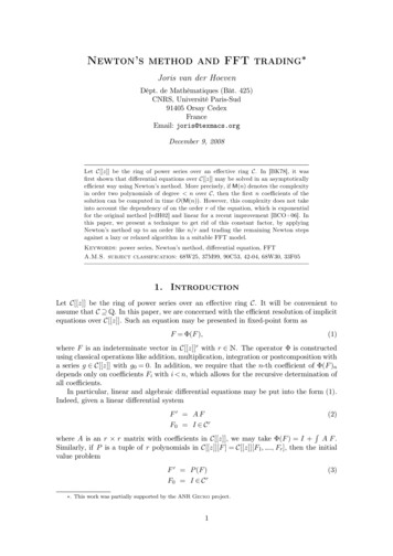
4Newton’s method and FFT trading 1so that (δ A)(M;n ) O(z 2n) and Mn;2n O(z 2n). Computing M;n and M;ntogether using (6) and the usual Newton iteration [Sch33, MC79] 1 1 1 1M;2n [M;n M;n(1 M;n M;n)];2n(7)for inverses yields an algorithm of time complexity O(MM(n, r)). The quantities En;2n andMn;2n n;2n may be computed efficiently using the middle product algorithm [HQZ04].Instead of doubling the precision at each step, we may also increment the number ofknown terms with a fixed number of terms m. More precisely, given n, m 0, we have 1)(δM;n A;n m M;n)];n m.M;n m 4 [M;n (M;m δ 1 M;m(8)This relation is proved in a similar way as (6). The same recurrence may also be appliedfor computing blocks of coefficients of the unique solution F C[[z]]r to the vector lineardifferential equation(9)δF A Fwith initial condition F0 I C r: 1F;n m 4 [F;n (M;m δ 1 M;m)(δF;n A;n m F;n)];n m.(10)Both the right-hand sides of the equations (8) and (10) may be computed efficiently usingthe middle product.Assume now that we want to compute F;n and take m n. For simplicity, we willassume that n k m with k N and that C contains all 2 p-th roots of unity for p N. Westart by decomposing F;n usingF;n F[0] F[k 1]F[i] Fim;(i 1)m(11)and similarly for A. Setting P A F , we haveP[i] (A[i 1] A[i]) F[0] (A[0] A[1]) F[i 1] (A[ 1] A[0]) F[i],where stands for the middle product (see figure 1). Instead of computing P[i] directly using this formula, we will systematically work with the FFT transforms F[j]of F[j] atorder 2 m and similarly for A[j 1] A[j] and P[j], so that P[i] (A[i 1] A[i]) F[0] (A[0] A[1]) F[i 1] (A[ 1] A[0]) F[i].Recall that we may resort to TFT transforms [vdH04, vdH05] if m is not a power of two. 1Now assume that M[0], M[0]andpreP[i] P[i] (A[ 1] A[0]) F[i] ((A[0] A[i]) (F[0] F[i 1]))[i]are known. Then the relation (10) yieldshipre 1.F[i] (M[0] δ 1 M[0])P[i][i](12) 1 preIn practice, we compute F[i] via X (M[0]P[i] )[i], Y δX and F[i] (M[0] Y )[i], using FFT 1multiplication. Here we notice that the FFT transforms of M[0] and M[0]only need to becomputed once.