Transcription
Avestia PublishingInternational Journal of Mechanical Engineering and MechatronicsVolume 1, Issue 1, Year 2012ISSN: 2929 -2724Article ID: 008, DOI: 10.11159/ijmem.2012.00866A Simple Algorithm to Relate Measured SurfaceRoughness to Equivalent Sand-grain RoughnessThomas Adams, Christopher GrantRose-Hulman Institute of Technology, Department of Mechanical Engineering5500 Wabash Ave., Terre Haute, Indiana, USAadams1@rose-hulman.edu; grantcl@rose-hulman.eduHeather WatsonJames Madison University, School of Engineering801 Carrier Drive, Harrisonburg, Virginia, USAwatsonhl@jmu.eduAbstract - One of the most important resources available inthe field of fluid mechanics, the Moody Chart gives Darcyfriction factor as a function of Reynolds number and relativeroughness. The experimentalists who generated the datacorrelated in the Moody Chart, however, roughened pipesurfaces by coating their internal surfaces with a monolayer ofsand, the pipe wall roughness being defined as the averagediameter of the sand grains. Thus, the sand-grain roughnessvalues required for use with the Moody Chart are not derivedfrom any direct measure of roughness using modern surfacecharacterization equipment, such as an optical profilometer.Using direct measurements of surface roughness in fluid flowcalculations may therefore result in significant error. In thispaper we present a simple algorithm with which variousmeasured surface roughness parameters can be converted toequivalent sand-grain roughness. For nearly every surfaceroughness value converted to equivalent sand-grain roughnessusing the algorithm, better agreement with fluid flowexperiments is seen over using the raw roughness value.Keywords: Surface Roughness, Sand-Grain Roughness,Moody Chart, Darcy Friction Factor Copyright 2012 Authors - This is an Open Access articlepublished under the Creative Commons AttributionLicense terms tricted use, distribution, and reproduction in any mediumare permitted, provided the original work is properly cited.1. IntroductionThe Moody Chart (Moody, 1944) represents one of themost widely used resources in fluid mechanics. RelatingDarcy friction factor to Reynolds number and relativeroughness, the Moody Chart correlates extensiveexperimental data obtained earlier by Nikuradse (1933), inwhich pipe surfaces were roughened by coating their internalsurfaces with a layer of sand. Pipe wall roughness, ε, was thusdefined as the average diameter of a sand grain. Actual pipesurfaces, however, do not have such a regular surfacegeometry as that created by a monolayer of sand grains.Rather, they are replete with hills and valleys of various sizesand shapes. Thus, direct measurements of surface roughnessmay not be appropriate for fluid flow calculations and couldlead to significant error. And though profilometry techniquesfor measuring surface roughness represent a maturetechnology, the algorithms employed for calculating anaverage roughness do not coincide with the idea of sandgrain roughness.Values of roughness reported in tables in fluid mechanicstexts and handbooks typically reflect an “equivalent sandgrain” idea of roughness, having been back-calculated bycomparing pressure drop data from fluid flow experiments tothe Moody Chart. These equivalent sand-grain roughnessvalues do not result from any direct measurement of surfaceroughness using standard surface characterizationequipment and the various definitions of surface roughnessthereof. When encountered with a pipe surface for which nosuch data exist, especially when utilizing new materialsand/or fabrication techniques, one usually measures surfaceroughness directly using any number of availableprofilometers. A link between measured surface roughness
67and the sand-grain roughness required for friction factorpurposes would therefore be highly useful.A number of researchers have recognized theshortcomings of using measured surface roughnessparameters in conjunction with the Moody Chart. The work ofKandlikar et al. (2005) was partly motivated by the very largerelative roughnesses (up to 14%) encountered inmicrochannels. They re-plotted the Moody Chart using theidea of a constricted flow diameter. Bahrami et al. (2005)assumed pipe wall roughness to have a Gaussian distribution,and found frictional resistance using the standard deviationin the roughness profile. Pesacreta and Farshad (2003)showed that measured peak-to-valley roughness, Rzd, betterrepresent sand-grain roughness than the more commonarithmetic average roughness, Ra. Taylor et al. (2005) givesan excellent review of much of this work.2. Proposed Roughness Conversion AlgorithmA simple solution to the problem or relating surfacemeasurements to sand grain roughness is to calculate theroughness of a hypothetical surface assuming it to be madeup of a uniform monolayer of same-diameter spheres whileemploying the same integration techniques as in standardprofilometer software. The resulting algebraic expressionscan then be inverted and solved for sphere diameter in termsof “measured” roughness. When applied to actual surfaceroughness measurements, these expressions give anapproximate value for equivalent sand-grain roughness.2. 1. Measured Surface Roughness ParametersA number of different parameters have been defined tocharacterize the roughness of surface such as that illustratedin Fig. 1. By far the most common is the arithmetic average ofabsolute values,1 nRa y i ,n i 1(1)where yi is the distance from the average height of a profile(the mean line) for measurement i, and n is the number ofmeasurements. Two other parameters considered in thepresent work are the root mean squared and the peak-tovalley values:RRMS Rzd 151nn y2,(2)i 1 R5ipi R vi .(3)yxMean lineFig. 1. A rough surface of arbitrary profile2. 2. Illustration of Conversion AlgorithmFigure 2 gives a schematic diagram of a single row ofspheres of diameter ε on a flat surface as viewed from theside. For a scan in the x-direction across the tops of thespheres, the surface as seen by a profilometer would appearas a uniform row of half-circles (Fig. 3). In the limit as thenumber of measurements goes to infinity, (1) becomes theintegralRa 1 x 0y y dx .(4)For the profile in Fig. 3y( x) x x 2(5)andy (6)8Substituting (5) and (6) into (4) and performing theintegration givesRa 1/ 2 2 cos 1 1 2 216 1/ 2 2 1 4 16 . Solving (7) for ε and simplifying givesε 11.03Ra.(8)Equation (8) shows that if a profilometer were used tomeasure Ra for a surface consisting of a layer of spheres ofdiameter ε, the resulting value of Ra could be as much as anorder of magnitude smaller than sand-grain roughnessappropriate for friction factor calculations.i 1In the peak-to-valley parameter Rpi and Rvi refer to the largestdistances above and below the mean line for one of fivemeasurements, all of equal scan length in the x-direction.(7)εFig. 2. A row of uniform spheres on a flat surface
684. Experimental ValidationyxFig. 3. The surface as seen by a profilometer3. Generalized AlgorithmIt is highly unlikely that a profilometer measuring theroughness of a surface comprised of a monolayer of uniformspheres would scan atop the peak of each sphere. Therefore,a more sophisticated model in which integrals of the typegiven in (4) can be performed for different scan directionswas developed using the software package MATLAB. Fig. 4shows a model of hexagonally packed spheres created inMATLAB for this purpose.In order to validate the estimates of ε given in Table 1, aA Zygo NewView 6300 interferometer was used to measureRa, RRMS, and Rzd for pipes of several different materials,including copper, aluminium, steel, and galvanized steel. Thevalues were then converted to their respective sand-grainroughness estimates given in Table 1 and then compared toequivalent sand-grain roughness values obtained fromturbulent fluid flow experiments performed on the samelength of pipe.4. 1. Fluid Flow ExperimentsExperimental values for equivalent sand-grainroughness were obtained for the various pipes via fluid flowexperiments. In effect, measured values of head loss and flowrate were used to calculate experimental values of frictionfactor and Reynolds number, which in turn were used in theequation developed by Haaland (1983) to estimateequivalent sand-grain roughness:1fFig. 4. Model of hexagonally packed spheres created in MATLABUsing the algorithm outlined in 2.2, the MATLAB modelwas used to relate Ra, RRMS, and Rzd as given in (1)-(3) to thediameter of the spheres, ε. For each parameter the MATLABmodel averaged scans made in three directions: atop thepeaks of each sphere, over the points of contact between thespheres (the lowest point), and midway between those twodirections. The results are given in Table 1.Table 1. Estimated sand-grain roughness based on measured surfaceroughness parameters.Roughness parameterEstimated sand-grainroughness, εRaRRMSRzdε 5.863Raε 3.100RRMSε 0.978Rzd / D 1.11 6.9 3.7 Re 1.8 log (9)The Haaland equation was used rather than other curve fitsfor the Moody Chart since the equation can be explicitlysolved for ε.Figure 5 gives a schematic diagram of the flow apparatusitself along with the physically measured parameters. Thevarious pipe materials and dimensions are given in Table 2,and typical values of the other measurands are given in Table3. Water at room temperature was used in all experiments.Time, thLDLCollectedvolume,Fig. 5. Fluid flow experiment to measure equivalent sand-grainroughness. A measured volume of water discharged to theatmosphere along with time measurements yielded flow rates.
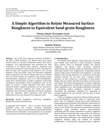
69Table 2. Pipe materials and dimensions.MaterialLength, L(cm)Diameter, D(cm)CopperCopperAluminiumSteelGalvanized steel (smooth)Galvanized steel 01.57Table 3. Typical measurand values for fluid flow experiments.Pipe materialLength, LPipe Diameter, DHead loss, hLVolume, Time, tCopper0.625 m0.02 m0.08 m0.0222 m330 sec4. 2. Results and DiscussionFigure 6 gives a comparison of the various roughnessvalues for the 2.05-cm diameter copper pipe obtained fromthe optical profilometer, the estimated sand-grain roughnessbased on those values using the algorithm, and the value ofequivalent sand-grain roughness found from the fluid flowexperiments. Circles represent roughness values obtainedfrom the profilometer, with filled-in circles giving thecorresponding estimated sand-grain roughness using thealgorithm. The shaded grey region on either side of themeasured sand-grain roughness indicates its experimentaluncertainty. The measured value of equivalent sand-grainroughness from the fluid flow experiments is considered thetrue value. Table 4 gives the corresponding numerical values.Standard uncertainty propagation techniques were used toestimate all experimental uncertainties.In order to reduce the data to find equivalent sand-grainroughness, experimental values of friction factor andReynolds number were determined first. Equations (10) and(11) give the familiar relations for head loss in terms offriction factor and Reynolds number, respectively:hL fL V2,D 2g(10) VDRe (11)where f is friction factor, ϱ, is density, and μ is viscosity. Interms of the measurands given in Tables 2 and 3, (10) and(11) can be rearranged to give the data reduction equationsfor f and Re as4 Re , Dtf 2 ghL D 5t8L 2.Table 4. Comparison of various roughness values.(12)Roughness parameter(13)Arithmetic average,RaRoot mean square,RRMSPeak-to-valley, RzdThese values were then used in the friction factor equationgiven in (9) and back-solved for ε to give the experimentalvalue of sand-grain roughness:1/1.111 1.8 f 6.9 3.7 D 10 expRe Fig. 6. Comparison of measured surface roughness, estimated sandgrain roughness obtained via the algorithm, and equivalent sandgrain roughness obtained from fluid flow experiments for 2.05-cmdiameter copper pipe.Equivalent sand-grainroughness from fluidflow experiment, εexp(14)Measuredvalue (μm)Estimatedsand-grainroughness(μm)0.2041.2 0.10.2690.8 0.11.891.85 0.091.78 0.08—Figure 6 and Table 4 show that of the measuredroughness parameters, Ra does the worst job of estimating
70equivalent sand-grain roughness and Rzd does the best. Oncethe algorithm is applied to a surface measurement, RRMS doesthe worst job of estimating ε, whereas Rzd again performs thebest. The superior estimate of ε resulting from the use of Rzdis consistent with previous research. By comparison, theexpected value for equivalent sand-grain roughness forcopper as given in Binder (1973) is 1.5 μm.In all cases, however, it should be noted that theconverted roughness values always come closer to the truevalue of sand-grain roughness than the raw measured values,with the converted value of Rzd falling within the range ofexperimental uncertainty of the true value.Figures 7-11 show the same comparisons for theremaining pipe materials and dimensions. The figures appearin order of increasing sand-grain roughness as obtained viaexperiment.Fig. 9. Comparison of roughness values for 1.55-cm steel pipe.Fig. 10. Comparison of roughness values for 2.10-cm galvanizedsteel pipe.Fig. 7. Comparison of roughness values for 1.44-cm copper pipe.Fig. 11. Comparison of roughness values for 1.57-cm galvanizedsteel pipe.Fig. 8. Comparison of roughness values for 4.22-cm aluminium pipe.Figures 7-11 all show the same trends as does Fig. 6 interms of raw measured surface parameters; that is, Ra doesthe worst job of estimating sand-grain roughness whereas Rzddoes the best. Furthermore, the estimated values of sandgrain roughness found by applying the algorithm to Ra andRRMS always come closer to ε than do the raw values, with theconverted Ra consistently outperforming the converted RRMS.Less consistent, however, are trends in Rzd. At lowervalues of sand-grain roughness Rzd under predicts ε, whereas
71at
measured surface roughness parameters can be converted to equivalent sand-grain roughness. For nearly every surface roughness value converted to equivalent sand-grain roughness using the algorithm, better agreement with fluid flow experiments is seen over using the raw roughness value.