WIXLIB

06 - Data Visualization (Part II)Data and Information EngineeringSYS 2202 Fall 201906-dataviz2.pdfContents1Cleveland Dot Plot1.1 Baseball Team Stats . . . . . . . . . . . . . . . . . . . . . . . . . . . . . . . . . . . . . . .1.2 Analyzing Hits . . . . . . . . . . . . . . . . . . . . . . . . . . . . . . . . . . . . . . . . .1.3 Cleveland Dot Plot Aesthetics . . . . . . . . . . . . . . . . . . . . . . . . . . . . . . . . .22242Line Graphs2.1 economics data . . . . . . . . . . . . . . . . . . . . . . . . . . . . . . . . . . . . . . . .2.2 Your Turn: Stock Price . . . . . . . . . . . . . . . . . . . . . . . . . . . . . . . . . . . . .558Required Packages and erse)# may need to: install.packages("tidyquant")# may need to: install.packages("Lahman")

06 - Data Visualization (Part II)1SYS 2202 Fall 20192/8Cleveland Dot PlotWilliam Cleveland wrote a popular book on visualizing data The Elements of Graphing Data that has manyuseful suggestions. One element he stressed was to reduce the cognitive strain on the view. One way to dothis is to use as little ink as possible. The Cleveland dot plot contains the same information as a bar graph,but instead of using all the ink needed for the bar, remove the bar altogether and place a dot at the bar height(using geom point()).1.1Baseball Team StatsConsider the baseball dataset Teams from the Lahman package. This gives the team performance by year.Your Turn #1 : Get Batting DataGet the team performance for year (yearID) 2018 (Boston Red Sox beat the LA Dodgers in the WorldSeries). Specifically, extract only the team name (name), league (lgID), wins (W), runs (R), at-bats (AB), hits (H),doubles (X2B), triples (X3B), home runs (HR), walks (BB); name the new object bat18 for (batting 2018)# Error in select(., name, lgID, W, R:BB): unused arguments (name, lgID, W, R:BB)The first few rows should look like this:1.2namelgIDWRABHX2BX3BHRBBX1BArizona DiamondbacksAtlanta BravesBaltimore OriolesBoston Red SoxChicago White SoxChicago 22569425576798915872915851966Analyzing HitsLet’s make the bar graphggplot(bat18) geom col(aes(x name, y H))1500H10005000Arizona lsTorontoBayWashingtonRangersRaysBlue JaysNationalsname

06 - Data Visualization (Part II)SYS 2202 Fall 20193/8This isn’t very revealing.1. I can’t see the team names2. There should be some ordering of data. ordering by Hits or Wins make more sense the the default (alphabetical)3. Because the y-axis starts at 0, the differences between teams is not very apparent.We can fix 1 and 2 very easily:ggplot(bat18) geom col(aes(x reorder(name, W), y H)) labs(x '', y 'Hits', title 'Team Hits, ordered by Wins (2018)') coord flip()Team Hits, ordered by Wins (2018)Boston Red SoxHouston AstrosNew York YankeesOakland AthleticsMilwaukee BrewersChicago CubsLos Angeles DodgersColorado RockiesCleveland IndiansTampa Bay RaysAtlanta BravesSeattle MarinersSt. Louis CardinalsWashington NationalsPittsburgh PiratesArizona DiamondbacksPhiladelphia PhilliesLos Angeles Angels of AnaheimMinnesota TwinsNew York MetsToronto Blue JaysSan Francisco GiantsTexas RangersCincinnati RedsSan Diego PadresDetroit TigersMiami MarlinsChicago White SoxKansas City RoyalsBaltimore Orioles050010001500Hits The function reorder() convert a vector into a factor and orders it according to a function of asecondary variable. Above, we order the teams according to wins (W). The function coord flip() swaps and x and y coordinates. Notice that the labs() arguments stillcorrespond to the non-flipped axes.Compare the bar graph with the dot plot.#- (left) bar graphggplot(bat18) geom col(aes(x reorder(name, W), y H)) labs(x '', y 'Hits', title 'Team Hits, ordered by Wins (2018)') coord flip()#- (right) corresponding dot plotggplot(bat18) geom point(aes(x reorder(name, W), y H)) labs(x '', y 'Hits', title 'Team Hits, ordered by Wins (2018)') coord flip()

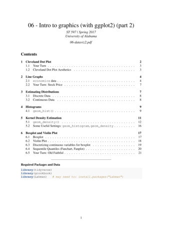
06 - Data Visualization (Part II)SYS 2202 Fall 2019Team Hits, ordered by Wins (2018)4/8Team Hits, ordered by Wins (2018)Boston Red SoxHouston AstrosNew York YankeesOakland AthleticsMilwaukee BrewersChicago CubsLos Angeles DodgersColorado RockiesCleveland IndiansTampa Bay RaysAtlanta BravesSeattle MarinersSt. Louis CardinalsWashington NationalsPittsburgh PiratesArizona DiamondbacksPhiladelphia PhilliesLos Angeles Angels of AnaheimMinnesota TwinsNew York MetsToronto Blue JaysSan Francisco GiantsTexas RangersCincinnati RedsSan Diego PadresDetroit TigersMiami MarlinsChicago White SoxKansas City RoyalsBaltimore OriolesBoston Red SoxHouston AstrosNew York YankeesOakland AthleticsMilwaukee BrewersChicago CubsLos Angeles DodgersColorado RockiesCleveland IndiansTampa Bay RaysAtlanta BravesSeattle MarinersSt. Louis CardinalsWashington NationalsPittsburgh PiratesArizona DiamondbacksPhiladelphia PhilliesLos Angeles Angels of AnaheimMinnesota TwinsNew York MetsToronto Blue JaysSan Francisco GiantsTexas RangersCincinnati RedsSan Diego PadresDetroit TigersMiami MarlinsChicago White SoxKansas City RoyalsBaltimore tsYour TurnYour Turn #2 : Dot Plot vs. Bar Plot1. What was changed in the code to make the Cleveland Dot Plot?2. What are the differences between the two plots?3. How would you add information about team homeruns to the bar plot? How about to the dotplot?1.3Cleveland Dot Plot AestheticsThe real strength Cleveland’s dotplot is in the ability to add additional aesthetics, like size, color, shape.Your Turn #3 : Dressing up, Cleveland StyleModify the dot plot by adding the following:1. Size the dots by runs (R)2. Color the dots by league (lgID)Final touches include changing the theme, modifying the colors and sizes#- new themedot theme theme bw() theme(panel.grid.major.x element blank(),panel.grid.minor.x element blank(),panel.grid.major.y element line(color "grey60",linetype "dotted"))#- Cleveland dot plotggplot(bat18) geom point(aes(x reorder(name, W), y H, size R, color lgID)) labs(x '', y 'Hits', title 'Team Hits, ordered by Wins (2018)') coord flip() dot theme scale color manual(name "League", values c("#002D72", "#D50032")) scale radius(name "Runs", range c(1,6))

06 - Data Visualization (Part II)SYS 2202 Fall 20195/8Team Hits, ordered by Wins (2018)Boston Red SoxHouston AstrosNew York YankeesOakland AthleticsMilwaukee BrewersChicago CubsLos Angeles DodgersColorado RockiesCleveland IndiansTampa Bay RaysAtlanta BravesRunsSeattle MarinersSt. Louis Cardinals600Washington Nationals700Pittsburgh Pirates800Arizona DiamondbacksLeaguePhiladelphia PhilliesLos Angeles Angels of AnaheimALMinnesota TwinsNLNew York MetsToronto Blue JaysSan Francisco GiantsTexas RangersCincinnati RedsSan Diego PadresDetroit TigersMiami MarlinsChicago White SoxKansas City RoyalsBaltimore Orioles13001350140014501500HitsThe Cleveland Dot Plot is an alternative to a bar plot. There is also a dot plot (geom dotplot()) that is analternative to a histogram.2Line Graphs2.1 economics dataThe economics data from the ggplot2 package contains some economic time series datalibrary(tidyverse)data(economics)# from the ggplot2 package (part of tidyverse package)glimpse(economics)# Observations: 574# Variables: 6# date date 1967-07-01, 1967-08-01, 1967-09-01, 1967-10-01, 1967.# pce dbl 507, 510, 516, 512, 517, 525, 531, 534, 544, 544, 550.# pop dbl 198712, 198911, 199113, 199311, 199498, 199657, 19980.# psavert dbl 12.6, 12.6, 11.9, 12.9, 12.8, 11.8, 11.7, 12.3, 11.7,.# uempmed dbl 4.5, 4.7, 4.6, 4.9, 4.7, 4.8, 5.1, 4.5, 4.1, 4.6, 4.4.# unemploy dbl 2944, 2945, 2958, 3143, 3066, 3018, 2878, 3001, 2877,.

06 - Data Visualization (Part II)SYS 2202 Fall 20196/8We can plot the number of unemployed over time with a line plot (using geom line())ggplot(economics, aes(date, unemploy)) geom eggplot() recognizes the date class and smartly adds yearly tick marks!We can fancy it up, maybe add some pointsggplot(economics, aes(date, unemploy)) geom line(size 2, color "orange") geom point(shape 21, color 'blue', fill 'white', size 1)unemploy1200080004000197019801990dateWe can shade the region under the line with geom area()20002010

06 - Data Visualization (Part II)SYS 2202 Fall 20197/8ggplot(economics, aes(date, unemploy)) geom area(color 'black', fill '#C28E0E', alpha .7, size 1)# Go 0dateMultiple lines (using another aesthetic mapping for second line)ggplot(economics, aes(date, unemploy)) geom line(size 2, color "orange") # uses y number of unemployedgeom line(aes(date, uempmed*1000 ))# uses y 1000* median duration of 80199020002010dateHow did the economy do for the presidents? Let’s use the presidential data from ggplot2 and usegeom rect() to shade in the time period for each presidentdata(presidential)ggplot(economics) # load the presidential data (from ggplot2/tidyverse)

06 - Data Visualization (Part II)SYS 2202 Fall 20198/8geom line(aes(date, unemploy),size 1.5, color "black") geom rect(data filter(presidential, start as.Date("1969-01-01")),aes(xmin start, xmax end, ymin -Inf, ymax Inf, fill reorder(name, start)),alpha .3) scale fill brewer(palette "Set1", name ate2.2Your Turn: Stock PriceYour Turn #4 : Stock PriceThis exercise will walk you through a simple way to plot stock data.1. The R package tidyquant provides quick access to daily stock price data. Install and loadthis package.2. Get the Netflix (NFLX) stock data for 2018 - present using the td get() function.library(tidyquant)# may need to install it firstNFLX tq get("NFLX", from "2018-01-01", to today()) # nifty today() function3. Examine the data, then create a line plot of the close price by date. Color the line darkgreen.4. Use geom area() to fill the area below the line with lightgreen.

1 Cleveland Dot Plot William Cleveland wrote a popular book on visualizing dataThe Elements of Graphing Datathat has many useful suggestions. One element he stressed was to reduce the cognitive strain on the view. One way to do this is to use as little ink as possible. The Cleveland dot plot contains the same information as a bar graph,