WIXLIB

2CHAPTER 1. INTRODUCTION AND OVERVIEWcompensation capacitor to move the zero from RPH to left-hand-plane (LPH), which is themost popular and straightforward method among all others [30]. Voltage Buffer and CurrentBuffer techniques are used to remove this RPH zero by blocking the feed-forward current flowin the compensation circuit. Moreover, all the design processes will also be discussed furtherregarding the performance improvement of compensated two-stage Op-Amp. The Cadencedesigns and simulation results have been obtained by TSMC 180nm CMOS technology. Allthe compensation designs will also be discussed and compared based on a given standardOp-Amp performance.1.2OverviewChapter 2 presents the significance of stability of Op-Amp and then states all the compensation techniques in the order of traditional Miller Compensation, Nulling Resistor, VoltageBuffer, and Current Buffer.Chapter 3 depicts the Cadence design procedures and demonstrates the simulation resultswhere evaluations, improvements, and comparisons among all techniques are stated.Chapter 4 draws a conclusion from all the works presented in the previous chapters.

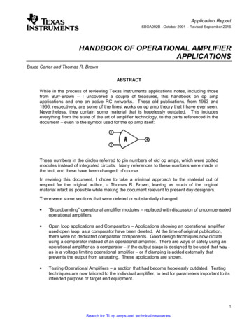
Chapter 2Background and Conceptual Principle2.1Background of Amplifier System StabilityTwo or more stages amplifiers can be implemented to achieve high gain and high output swingregardless of the limitations of the power supply voltage or power consumption comparedto single stage amplifiers. However, multiple stage amplifiers are generally complicated tocompensate. An uncompensated two-stage operational amplifier has a two-pole transferfunction, and both poles are located below the unity gain frequency.Figure 2.1: Block diagram of a Miller compensated operational amplifier [8]Therefore, a compensation circuitry must be implemented to enlarge the phase margin so3

4CHAPTER 2. BACKGROUND AND CONCEPTUAL PRINCIPLEdoes the stability, which will be talked further in this chapter. This compensation circuitrycan also be called as a compensator or a feedback network in operational amplifiers design.As shown in the Figure 2.1, the Miller capacitor is used as a negative feedback network tocompensate the system, which feeds a current back from the output to the middle of the twostages A1 and A2.Figure 2.2: Block Diagram of a Single Loop Feedback SystemHowever, Operational amplifiers operating on a close-loop with a negative-feedback systemare susceptible to oscillation. The more oscillation it generates to the output, the moreunstable the system is. Figure 2.2 depicts a general block diagram of an amplifier system witha single feedback network, which closely represents the compensated two-stage operationalamplifier shown in Figure 2.1. In Figure 2.2, A(s) indicates the differential voltage gain ofthe operational amplifier, and F(s) indicates the feedback transfer function from the outputback to the input. Some important loop gain definitions are shown in the following Equation2.1 and 2.2:OpenLoopGain L(s) A(s)F (s)CloseLoopGain A(s)V out(s) V in(s)1 A(s)F (s) A(jω1 )F (ω1 ) 1(2.1)(2.2)(2.3)

2.1. BACKGROUND OF AMPLIFIER SYSTEM STABILITY A(ω1 )F (ω1 ) 180 5(2.4)According to the Barkhausen’s Criterion, the oscillation condition of such system needs tomeet two requirements which are represented in Equation 2.3 and 2.4, where F(s) here isconsidered as a constant [29]. The total phase shift of the system is 360 at ω1 because thenegative feedback network introduces a 180 phase shift. In this case, the circuit can amplifyits own noise until it eventually begins to oscillate at frequency ω1 [29].Figure 2.3: Phase Margin Demonstration [8]P haseM argin ϕM Arg[ A(jω0dB )F (jω0dB )] Arg[L(jω0dB )](2.5)One major criterion to measure the stability of this system is the phase margin, which is thephase angle difference from the 0dB frequency to 180 as shown in Equation 2.5 [7]. Phasemargin indicates system relative stability, and the tendency of oscillation during its responseto an input change such as a step function. Consider a step response of the second-ordersystem which models the closed-loop gain of the two-stage operational amplifier. Shown onFigure 2.3, smaller phase margin tends to have larger overshoot and longer settling time to a

6CHAPTER 2. BACKGROUND AND CONCEPTUAL PRINCIPLEstep response input while larger phase margin can settle the output down quicker and has lessoutput oscillation. For most of the two-stage Op-Amp, designers want to settle the outputdown quickly instead of letting it oscillate, so a large phase margin of a system is preferred,which should be at least 45 and preferable 60 or larger. Also, too much overshoot has arisk of damaging the output device.Figure 2.4: Uncompensated Frequency Response of Two Stage Operational Amplifier [8]Shown in Figure 2.4, the phase margin at ω0dB is close to 0 due to the two poles, which isgenerated by the two stage amplifier, are below the unity gain frequency. Even though p2is close to the unity gain frequency, it nearly drops another 90 to the phase margin. Dueto this major issue, the amplifier must have a compensation network to enlarge its phasemargin to at least 45 to ensure the stability of the whole system. One of the most commonapproaches to address this issue is called Miller Compensation.

72.2. COMPENSATED OP-AMP SURVEY2.2Compensated Op-Amp SurveyBefore talking about the Miller compensation and all other techniques, a summarized surveyis listed below which includes and compares all the related topologies of compensations. Thissurvey compares some typical compensation designs including Miller Compensation, Millercompensation with Nulling resistor, and Current buffer.Referredpaper workMillercompensation[25]Miller compensationwith Nullingresistor[35]Currentbuffer[28]Supply Voltage(V)DC Gain(dB)Gain Bandwidth(MHz)Phase Margin( )Slew Rate(V/µs)Power Consumption (µW)CMRR(dB)PSRR(dB)2.9 - 1-3.378.215.8263.975.58144.3489.05117.73Table 2.1: Survey of various op amps topologiesCommon mode rejection ratio (CMRR) is measured by: differential gain – common modegain, where differential gain is the DC gain [29], [25]. By applying this equation to allthree works, we can know the typical common mode gain range is around 4dB to 10dB.Power supply rejection ratio (PSRR) measures the power supply noise rejection ability ofthe amplifier, which are pretty high for all three designs ( over 80dB ). Due to the similarityand stability of CMRR and PSRR of two-stage operational amplifier, this two parameterswill not be considered in the design and simulation in Chapter 3.

82.3CHAPTER 2. BACKGROUND AND CONCEPTUAL PRINCIPLEMiller Compensation Technique PrincipleMiller compensation is one of the most popular techniques that is used to increase the stability of the Multi-stage amplifier. The design that is shown in Figure 2.5 is the configurationof Miller compensation. The first stage of this Op-Amp consists of NMOS differential inputswith a PMOS current mirror load, whereas the second stage is a PMOS common sourceamplifier with a NMOS current mirror load. The compensation capacitor is connected between the output of these two stages, so this Compensation Capacitor CC is also called aMiller Capacitor [12] [33] [32]. This typology can also be referred as a single capacitor Millercompensation (SCMC) in some paper works [9]. Due to the direct connection of output andinput of the second stage, SCMC can also be called as Direct Feedback Compensation [34].The working principle of Miller compensation is to split the poles so a higher phase margincan be reached at the unity gain frequency [34]. However, a right-hand-plane (RHP) zero wasgenerated due to a feed forward current from the output of the first stage to the output ofthe second stage [10]. Before compensating the circuit, the two stage operational amplifierhas two poles which are located at p1 1,R 1 C1and p2 1,R2 C2where R and C are theresistance and capacitance respectively at the corresponding nodes shown in the Figure 2.6.The capacitors C1 and C2 are mainly formed by the parasitic capacitance of correspondingconnected MOSFETs of each node. After the implementation of the Miller Capacitor, thedominant pole and non-dominant pole are achieved due to the pole splitting. By using nodalanalysis at both input (V1 ) and output (V2 ) nodes of the common source stage, the systemgain equation can be generated as shown in equation 2.6, where the new positions of poles

2.3. MILLER COMPENSATION TECHNIQUE PRINCIPLE9Figure 2.5: Two-Stage Op-Amp with Miller Compensationand zero can also be found.cgm1 gm7 R1 R2 (1 gsC)V out(s)m7AV (s) V in(s)1 sa s2 ba (C2 CC )R2 (C1 CC )R1 gm7 R1 R2 CC ,(2.6)b R1 R2 (C1 C2 C1 CC C2 CC )In equation 2.6, the DC gain and the position of zero can be noticed directly. The amplifierDC gain is:DCgain gm1 gm7 R1 R2(2.7)

10CHAPTER 2. BACKGROUND AND CONCEPTUAL PRINCIPLEFigure 2.6: Small Signal Model of Miller Compensation TechniqueThe value of the RPH zero is:z1 gm7CC(2.8)To find the new positions of both poles, the denominator needs to be simplified. Assumethe denominator of AV (s) is D(s). In general, for quadratic equation like D(s), it can berewrote to the following form:ss)(1 )p1p211s2 1 s( ) p1 p2p1 p22ss f or p1 p2 1 p1 p1 p2D(s) (1 (2.9)In order to get the precise and the simplified value of p1 and p2 , the equation 2.9 needs tobe matched with the denominator of the equation 2.6. So the value of the dominant pole p1

2.3. MILLER COMPENSATION TECHNIQUE PRINCIPLE11is: 1(C2 CC )R2 (C1 CC )R1 gm7 R1 R2 CC 1 gm7 R1 R2 CCp1 (2.10)The value of the non-dominant p2 is:(C2 CC )R2 (C1 CC )R1 gm7 R1 R2 CCR1 R2 (C1 C2 C1 CC C2 CC )gm7 CC C1 C2 C1 CC C2 CCgm7gm7 or, f or C2 CC C1 C2 C1C2p2 (2.11)As shown in Figure 2.7, the original open-loop poles p′1 , and p′2 are split to the new positionFigure 2.7: Pole Splitting Demonstration [2]p1 and p2 due to the Miller Compensation, where their values are shown in Equation 2.10and 2.11. p1 becomes more dominant than it used to be, which results in the system startingto behave as a first order system in low frequency range. On the contrary, p2 moves tothe other direction which makes it more non-dominant. The goal of splitting both poles isachieved, however, a RHP zero z1 is generated, which is undesirable because it boosts the

12CHAPTER 2. BACKGROUND AND CONCEPTUAL PRINCIPLEgain while decreasing the phase [22] [34]. One approach to address this issue is to make sureits frequency is 10 times larger than the unity gain bandwidth frequency by adjusting thecorresponding parameter of z1 which is shown in Equation 2.8. This is the main reason thatthe size of the compensation capacitor cannot be too large. To ensure at least 45 phasemargin, the effective frequency of the second pole p2 must be the same or larger than theunity gain bandwidth as illustrated in the Figure 2.8. To obtain a higher phase margin, p2needs to be moved to the left further in Figure 2.7 which is the high-frequency direction inFigure 2.8, so that p2 has less effect of reducing the phase margin.Figure 2.8: Compensated Frequency Response of Two Stage Operational Amplifier [2]So the key point for now is to find the unity gain bandwidth shown as ‘GB’ in Figure 2.8,which is the value of 0dB frequency. In this graph, the location of ‘GB’ is only affected bythe value of the dominant pole p1 , where the gain starts to drop as a slope of -20dB/decade.

2.3. MILLER COMPENSATION TECHNIQUE PRINCIPLE13So the relationship of these variables can be derived as the equation below:20log10 (AV (0)) [log10 (GB) log10 ( p1 )] 20log10 (AV (0)) log10 (GB) p1 GB AV (0) p1 (2.12)gm1 gm7 R1 R2gm7 R1 R2 CCgm1GB CCGB Suppose the required phase margin for stability is 60 , then the location of p2 can be estimated from this phase requirement by using the following equation:180 tan 1ωωω tan 1 tan 1 P M 60 p1 p2 z1 (2.13)Let ω be equal to the unity gain bandwidth frequency GB in the previous equation andassume z1 is 10 times larger than GB, then the following equation can be obtained [2]. Themain reason to let z1 10 times larger than GB is to shrink its effect of phase margin.GBGBGB tan 1 tan 1 P M 60 p1 p2 z1 GB tan 1 (0.1) 60 180 tan 1 AV (0) tan 1 p2 GB180 90 60 5.7 tan 1 p2 GBGBtan 1 24.3 0.452 p2 p2 180 tan 1(2.14) p2 2.215 GBThen the relationship of the trans-conductance gm of Mosfets can be obtained by applyingthe Equation 2.8, 2.11, and 2.12 to the assumption above. The relationship between gm7

14CHAPTER 2. BACKGROUND AND CONCEPTUAL PRINCIPLEand gm1 is restricted by the assumption that z1 is 10 times larger than GB, which is shownin the following equation.z1 10 GBgm7gm1 10 CCCC(2.15)gm7 10gm1The value of the compensation capacitor CC can be estimated through the relationshipbetween p2 and GB that is shown in Equation 2.16. Knowing that C2 is the capacitancecorresponding to the output node which parasitic capacitances are relatively small comparedwith the load capacitor CL , so we can assume C2 is equal to the load capacitor for easycalculations. p2 2.215 GBgm1gm7 2.215 C2CC10gm1gm1 2.215 C2CC(2.16)CC 0.2215CLOverall, to obtain a phase margin at least 60 for stability, CC needs to be the same or largerthan the 0.2215 times C2 . Also, gm7 needs to be at least 10 times of gm1 . The positions ofboth poles and zero should be at the correct locations with respect to unity gain frequency.However, there are still several trade-offs in real world design of Two Stage Amplifiers. Forexample, increasing gm7 can separate the poles more but costs more power. Making the CCtoo large may not help with the phase margin as ωz1 will reduce too. Large CC could also

152.4. NULLING RESISTOR TECHNIQUE PRINCIPLEreduce the unity gain bandwidth. So to obtain a better stability of two-stage Op-Amps, theRHP zero must be addressed. There are several ways to get rid of this RHP zero, and oneof the most common approaches is adding Nulling Resistor which could move this zero fromthe right plane to the left [22].2.42.4.1Nulling Resistor Technique PrincipleNulling Resistor Technique BackgroundAs talked in the last section, adding a nulling resistor in series with the compensationcapacitor is one of the most common approaches to eliminate the negative effect of the RHPzero by moving this zero to the LHP [21] [17] [14] [11]. Figure 2.10 depicts the pole splittingphenomenon and shows all the locations of poles and zero. This nulling resistor RZ caneither be an actual resistor or a transistor as shown in Figure 2.9.(a) Nulling Resistor with Actual ResistorThe transistor used in(b) Nulling Resistor with TransistorFigure 2.9: Compensated Two-Stage Op-Amp with Nulling ResistorFigure 2.9b is PMOS, which can also be replaced by a NMOS transistor by connecting its

16CHAPTER 2. BACKGROUND AND CONCEPTUAL PRINCIPLEFigure 2.10: Locations of Ploes and the Zero [22]gate terminal to V dd. Instead of using a single transistor here, a CMOS switch can be usedto avoid dynamic range limitation in some specific applications [18]. This CMOS technologyswitch is also known as a Transmission Gate that connects a NMOS and a PMOS transistorin parallel as illustrated in Figure 2.11.Figure 2.11: Transmission Gate [18]For this configuration, when Q is low, both transistors are off, and the transmission gate isoff. When Q is high, both transistors are on, creating a low resistance close loop circuit. Soin this case, the signal Q is connected to a high voltage node which is usually the V dd whilethe signal Q is connected to a low voltage node which is always the ground. The resistancevalues of the both PMOS and NMOS are obtained from Equation 2.17 and 2.18, which arederived in [29].

172.4. NULLING RESISTOR TECHNIQUE PRINCIPLERON ROP 1µn Cox W(VGSL VT Hn )1(VSGµp Cox WL VT Hp )(2.17)(2.18)For the PMOS and the NMOS transistors in this transmission gate, their overdrive voltagesare much bigger than the absolute value of their drain to source voltages ( Vds ). So bothtransistors work in deep triode regions which operate like voltage controlled resistors [29].In this situation, the overdrive voltage is nearly stable so the resistance value can only bechanged by adjusting the parameterWLbased on the Equation 2.17 and 2.18. Both equationsalso work for a single MOSFET that is used as a nulling resistor in the compensation network.2.4.2Nulling Resistor Technique Frequency ResponseSimilar to the Miller Compensation Technique, to know the effect of the adding resistor, weneed to find all the poles and zeros through the small signal analysis. By applying nodalFigure 2.12: Small Signal Model of Nulling Resistor Techniqueanalysis to both V1 and Vout nodes in Figure 2.12, the relationship of output and input signalscan be derived, where we can find all the poles and zeros. The derivation is nearly the same

18CHAPTER 2. BACKGROUND AND CONCEPTUAL PRINCIPLEas the Miller Compensation Technique that is fully described in Section 2.3. The locationsof both original poles are the same as Miller Compensation Technique that are listed inEquation 2.10 and 2.11 which are p1 1gm7 CC R1 R2and p2 gm7.C2The new position of zerois given in the following equation [34].z1 1( gm71 RZ )CC(2.19)RZ is the resistance value of the nulling resistor. For RZ 1,gm7this zero will appear inLHP, which helps improve the phase margin thus the stability. This zero will vanish if RZ isequal to1gm7[18]. In fact, this resistor value can be further increased to place the z1 on topof the p2 which can eliminate its negative effect on phase margin.Figure 2.13: Frequency Response of the Miller Compensated Operational Amplifier withNulling Resistor [34]Another high-frequency pole p3 is introduced at p3 1RZ C1which is far away from bothp1 and p2 [34] [18] [22]. Considering RZ and C1 are relatively small compared with thevalue of other resistors and capacitors, the effects of this newly introduced pole will notbe considered in the Cadence design in Chapter 3. Figure 2.13 shows a sample frequencyresponse of a Miller compensated Op-Amp with nulling resistor, where the locations of unitygain frequency, p2 , p3 , and z1 are marked. This plot can also prove the above statement

2.5. VOLTAGE BUFFER TECHNIQUE PRINCIPLE19regarding p3 , as the value of p3 is over 100 times away from the unity gain frequency.2.5Voltage Buffer Technique PrincipleInstead of changing the location of the RHP zero, a voltage buffer can be used to eliminatethis zero by rejecting the feed-forward path through the Miller Capacitor in the feedback path[24] [16]. At the same time

Two-Stage Operational Amplifier Design by Using Direct and Indi-rect Feedback Compensations Jiayuan Zhang (ABSTRACT) This paper states the stability requirements of the amplifier system, and then presents, and