Transcription
CS490D:Introduction to Data MiningChris CliftonJanuary 23, 2004Data PreparationData Preprocessing Why preprocess the data?Data cleaningData integration and transformationData reductionDiscretization and concept hierarchygeneration SummaryCS490D21
Why Data Preprocessing? Data in the real world is dirty– incomplete: lacking attribute values, lacking certainattributes of interest, or containing only aggregatedata e.g., occupation “”– noisy: containing errors or outliers e.g., Salary “-10”– inconsistent: containing discrepancies in codes ornames e.g., Age “42” Birthday “03/07/1997” e.g., Was rating “1,2,3”, now rating “A, B, C” e.g., discrepancy between duplicate recordsCS490D3Why Is Data Dirty? Incomplete data comes from– n/a data value when collected– different consideration between the time when thedata was collected and when it is analyzed.– human/hardware/software problems Noisy data comes from the process of data– collection– entry– transmission Inconsistent data comes from– Different data sources– Functional dependency violationCS490D42
Why Is Data PreprocessingImportant? No quality data, no quality mining results!– Quality decisions must be based on quality data e.g., duplicate or missing data may cause incorrect or evenmisleading statistics.– Data warehouse needs consistent integration ofquality data Data extraction, cleaning, and transformationcomprises the majority of the work of building adata warehouse. —Bill InmonCS490D5Multi-Dimensional Measureof Data Quality A well-accepted multidimensional onsistencyTimelinessBelievabilityValue addedInterpretabilityAccessibility Broad categories:– intrinsic, contextual, representational, andaccessibility.CS490D63
Major Tasks in DataPreprocessing Data cleaning– Fill in missing values, smooth noisy data, identify or removeoutliers, and resolve inconsistencies Data integration– Integration of multiple databases, data cubes, or files Data transformation– Normalization and aggregation Data reduction– Obtains reduced representation in volume but produces thesame or similar analytical results Data discretization– Part of data reduction but with particular importance, especiallyfor numerical dataCS490D7Data Preprocessing Why preprocess the data?Data cleaningData integration and transformationData reductionDiscretization and concept hierarchygeneration SummaryCS490D94
Data Cleaning Importance– “Data cleaning is one of the three biggest problems indata warehousing”—Ralph Kimball– “Data cleaning is the number one problem in datawarehousing”—DCI survey Data cleaning tasks––––Fill in missing valuesIdentify outliers and smooth out noisy dataCorrect inconsistent dataResolve redundancy caused by data integrationCS490D10Missing Data Data is not always available– E.g., many tuples have no recorded value for severalattributes, such as customer income in sales data Missing data may be due to– equipment malfunction– inconsistent with other recorded data and thusdeleted– data not entered due to misunderstanding– certain data may not be considered important at thetime of entry– not register history or changes of the data Missing data may need to be inferred.CS490D115
How to Handle MissingData? Ignore the tuple: usually done when class label ismissing (assuming the tasks in classification—noteffective when the percentage of missing values perattribute varies considerably. Fill in the missing value manually: tedious infeasible? Fill in it automatically with– a global constant : e.g., “unknown”, a new class?!– the attribute mean– the attribute mean for all samples belonging to the same class:smarter– the most probable value: inference-based such as Bayesianformula or decision treeCS490D12Noisy Data Noise: random error or variance in a measured variable Incorrect attribute values may due to–––––faulty data collection instrumentsdata entry problemsdata transmission problemstechnology limitationinconsistency in naming convention Other data problems which requires data cleaning– duplicate records– incomplete data– inconsistent dataCS490D136
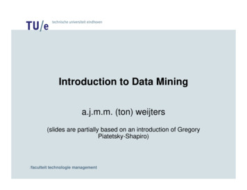
How to Handle Noisy Data? Binning method:– first sort data and partition into (equi-depth) bins– then one can smooth by bin means, smooth by binmedian, smooth by bin boundaries, etc. Clustering– detect and remove outliers Combined computer and human inspection– detect suspicious values and check by human (e.g.,deal with possible outliers) Regression– smooth by fitting the data into regression functionsCS490D14Simple DiscretizationMethods: Binning Equal-width (distance) partitioning:– Divides the range into N intervals of equal size: uniform grid– if A and B are the lowest and highest values of the attribute, thewidth of intervals will be: W (B –A)/N.– The most straightforward, but outliers may dominatepresentation– Skewed data is not handled well. Equal-depth (frequency) partitioning:– Divides the range into N intervals, each containing approximatelysame number of samples– Good data scaling– Managing categorical attributes can be tricky.CS490D157
Binning Methods for DataSmoothing Sorted data (e.g., by price) Partition into (equi-depth) bins:– 4, 8, 9, 15, 21, 21, 24, 25, 26, 28, 29, 34– Bin 1: 4, 8, 9, 15– Bin 2: 21, 21, 24, 25– Bin 3: 26, 28, 29, 34 Smoothing by bin means:– Bin 1: 9, 9, 9, 9– Bin 2: 23, 23, 23, 23– Bin 3: 29, 29, 29, 29 Smoothing by bin boundaries:– Bin 1: 4, 4, 4, 15– Bin 2: 21, 21, 25, 25– Bin 3: 26, 26, 26, 34CS490D16Cluster AnalysisCS490D178
RegressionyY1y x 1Y1’X1CS490Dx18Data Preprocessing Why preprocess the data?Data cleaningData integration and transformationData reductionDiscretization and concept hierarchygeneration SummaryCS490D199
Data Integration Data integration:– combines data from multiple sources into a coherent store Schema integration– integrate metadata from different sources– Entity identification problem: identify real world entities frommultiple data sources, e.g., A.cust-id B.cust-# Detecting and resolving data value conflicts– for the same real world entity, attribute values from differentsources are different– possible reasons: different representations, different scales, e.g.,metric vs. British unitsCS490D20Handling Redundancy in DataIntegration Redundant data occur often when integration ofmultiple databases– The same attribute may have different names indifferent databases– One attribute may be a “derived” attribute in anothertable, e.g., annual revenue Redundant data may be able to be detected bycorrelational analysis Careful integration of the data from multiplesources may help reduce/avoid redundanciesand inconsistencies and improve mining speedand qualityCS490D2110
Data Transformation Smoothing: remove noise from data Aggregation: summarization, data cubeconstruction Generalization: concept hierarchy climbing Normalization: scaled to fall within a small,specified range– min-max normalization– z-score normalization– normalization by decimal scaling Attribute/feature construction– New attributes constructed from the given onesCS490D22Data Transformation:Normalization min-max normalizationv' v minA(new maxA new minA) new minAmaxA minA z-score normalizationv' v mean Astand dev A normalization by decimal scalingv' v10 jWhere j is the smallest integer such that Max( v' ) 1CS490D2311
Z-Score oduction to Data MiningChris CliftonJanuary 26, 2004Data Preparation12
Data Preprocessing Why preprocess the data?Data cleaningData integration and transformationData reductionDiscretization and concept hierarchygeneration SummaryCS490D26Data Reduction Strategies A data warehouse may store terabytes of data– Complex data analysis/mining may take a very long time to runon the complete data set Data reduction– Obtain a reduced representation of the data set that is muchsmaller in volume but yet produce the same (or almost the same)analytical results Data reduction strategies–––––Data cube aggregationDimensionality reduction — remove unimportant attributesData CompressionNumerosity reduction — fit data into modelsDiscretization and concept hierarchy generationCS490D2713
Data Cube Aggregation The lowest level of a data cube– the aggregated data for an individual entity of interest– e.g., a customer in a phone calling data warehouse. Multiple levels of aggregation in data cubes– Further reduce the size of data to deal with Reference appropriate levels– Use the smallest representation which is enough tosolve the task Queries regarding aggregated informationshould be answered using data cube, whenpossibleCS490D28Dimensionality Reduction Feature selection (i.e., attribute subset selection):– Select a minimum set of features such that the probabilitydistribution of different classes given the values for thosefeatures is as close as possible to the original distribution giventhe values of all features– reduce # of patterns in the patterns, easier to understand Heuristic methods (due to exponential # of choices):––––step-wise forward selectionstep-wise backward eliminationcombining forward selection and backward eliminationdecision-tree inductionCS490D2914
Example ofDecision Tree InductionInitial attribute set:{A1, A2, A3, A4, A5, A6}A4 ?A6?A1?Class 1 Class 2Class 1Class 2Reduced attribute set: {A1, A4, A6}CS490D30Data Compression String compression– There are extensive theories and well-tuned algorithms– Typically lossless– But only limited manipulation is possible without expansion Audio/video compression– Typically lossy compression, with progressive refinement– Sometimes small fragments of signal can be reconstructedwithout reconstructing the whole Time sequence is not audio– Typically short and vary slowly with timeCS490D3215
Data CompressionCompressedDataOriginal DatalosslesssylosOriginal Daubechie4 Discrete wavelet transform (DWT): linear signalprocessing, multiresolutional analysis Compressed approximation: store only a small fraction ofthe strongest of the wavelet coefficients Similar to discrete Fourier transform (DFT), but betterlossy compression, localized in space Method:– Length, L, must be an integer power of 2 (padding with 0s, whennecessary)– Each transform has 2 functions: smoothing, difference– Applies to pairs of data, resulting in two set of data of length L/2– Applies two functions recursively, until reaches the desiredlengthCS490D3416
DWT for ImageCompression ImageLow PassLow PassLow PassHigh PassHigh PassHigh PassCS490D35Principal ComponentAnalysis Given N data vectors from k-dimensions, find c k orthogonal vectors that can be best used torepresent data– The original data set is reduced to one consisting of Ndata vectors on c principal components (reduceddimensions) Each data vector is a linear combination of the cprincipal component vectors Works for numeric data only Used when the number of dimensions is largeCS490D3617
Principal Component AnalysisX2Y1Y2X1CS490D37Numerosity Reduction Parametric methods– Assume the data fits some model, estimatemodel parameters, store only the parameters,and discard the data (except possible outliers)– Log-linear models: obtain value at a point inm-D space as the product on appropriatemarginal subspaces Non-parametric methods– Do not assume models– Major families: histograms, clustering,samplingCS490D3818
Regression and Log-LinearModels Linear regression: Data are modeled to fita straight line– Often uses the least-square method to fit theline Multiple regression: allows a responsevariable Y to be modeled as a linearfunction of multidimensional feature vector Log-linear model: approximates discretemultidimensional probability distributionsCS490D39Regress Analysis and LogLinear Models Linear regression: Y α β X– Two parameters , α and β specify the line and are tobe estimated by using the data at hand.– using the least squares criterion to the known valuesof Y1, Y2, , X1, X2, . Multiple regression: Y b0 b1 X1 b2 X2.– Many nonlinear functions can be transformed into theabove. Log-linear models:– The multi-way table of joint probabilities isapproximated by a product of lower-order tables.– Probability: p(a, b, c, d) αab βacχad δbcd19
Histograms A popular data reductiontechnique Divide data into bucketsand store average (sum)for each bucket Can be constructedoptimally in onedimension using dynamicprogramming Related to quantizationproblems.403530252015105010000 20000 30000 40000 50000 60000 70000 80000 90000 100000CS490D41Clustering Partition data set into clusters, and onecan store cluster representation only Can be very effective if data is clusteredbut not if data is “smeared” Can have hierarchical clustering and bestored in multi-dimensional index treestructures There are many choices of clusteringdefinitions and clustering algorithms,further detailed in Chapter 8CS490D4220
Sampling Allow a mining algorithm to run in complexity that ispotentially sub-linear to the size of the data Choose a representative subset of the data– Simple random sampling may have very poor performance in thepresence of skew Develop adaptive sampling methods– Stratified sampling: Approximate the percentage of each class (or subpopulation ofinterest) in the overall database Used in conjunction with skewed data Sampling may not reduce database I/Os (page at atime).CS490D43SamplingWORSRS le randomtp(sim le withousamp ment)cereplaSR SWRaw DataRCS490D4421
SamplingCluster/Stratified SampleRaw DataCS490D45Hierarchical Reduction Use multi-resolution structure with different degrees ofreduction Hierarchical clustering is often performed but tends todefine partitions of data sets rather than “clusters” Parametric methods are usually not amenable tohierarchical representation Hierarchical aggregation– An index tree hierarchically divides a data set into partitions byvalue range of some attributes– Each partition can be considered as a bucket– Thus an index tree with aggregates stored at each node is ahierarchical histogramCS490D4622
Data Preprocessing Why preprocess the data?Data cleaningData integration and transformationData reductionDiscretization and concept hierarchygeneration SummaryCS490D47Discretization Three types of attributes:– Nominal — values from an unordered set– Ordinal — values from an ordered set– Continuous — real numbers Discretization:– divide the range of a continuous attribute intointervals– Some classification algorithms only accept categoricalattributes.– Reduce data size by discretization– Prepare for further analysisCS490D4823
Discretization and Concepthierachy Discretization– reduce the number of values for a givencontinuous attribute by dividing the range ofthe attribute into intervals. Interval labels canthen be used to replace actual data values Concept hierarchies– reduce the data by collecting and replacinglow level concepts (such as numeric valuesfor the attribute age) by higher level concepts(such as young, middle-aged, or senior)CS490D49CS490D:Introduction to Data MiningChris CliftonJanuary 28, 2004Data Preparation24
Discretization and Concept HierarchyGeneration for Numeric Data Binning (see sections before)Histogram analysis (see sections before)Clustering analysis (see sections before)Entropy-based discretizationSegmentation by natural partitioningCS490D51Definition of Entropy EntropyH(X ) P( x) logx AX2P( x) Example: Coin Flip––––AX {heads, tails}P(heads) P(tails) ½½ log2(½) ½ * - 1H(X) 1 What about a two-headed coin? Conditional Entropy: H ( X Y ) P( y ) H ( X y )y AYCS490D5225
Entropy-BasedDiscretization Given a set of samples S, if S is partitioned into twointervals S1 and S2 using boundary T, the entropy afterpartitioning is S S H (S , T ) 1 S H ( S 1) 2 S H ( S 2) The boundary that minimizes the entropy function overall possible boundaries is selected as a binarydiscretization. The process is recursively applied to partitions obtaineduntil some stopping criterion is met, e.g.,H (S ) H (T , S ) δ Experiments show that it may reduce data size andimprove classification accuracyCS490D53Segmentation by NaturalPartitioning A simply 3-4-5 rule can be used to segmentnumeric data into relatively uniform, “natural”intervals.– If an interval covers 3, 6, 7 or 9 distinct values at themost significant digit, partition the range into 3 equiwidth intervals– If it covers 2, 4, or 8 distinct values at the mostsignificant digit, partition the range into 4 intervals– If it covers 1, 5, or 10 distinct values at the mostsignificant digit, partition the range into 5 intervalsCS490D5426
Example of 3-4-5 RulecountStep 1:Step 2:- 351- 159MinLow (i.e, 5%-tile)msd 1,000profitLow - 1,000 1,838High(i.e, 95%-0 tile) 4,700MaxHigh 2,000(- 1,000 - 2,000)Step 3:(- 1,000 - 0)(0 - 1,000)( 1,000 - 2,000)(- 4000 - 5,000)Step 4:(- 400 - 0)( 1,000 - 2, 000)(0 - 1,000)(0 200)(- 400 - 300)(- 300 - 200)(- 200 - 100)(- 100 0)( 1,000 1,200)( 200 400)( 1,200 1,400)( 1,400 1,600)( 400 600)( 600 800)( 800 1,000)CS490D( 1,600 ( 1,800 1,800) 2,000)( 2,000 - 5, 000)( 2,000 3,000)( 3,000 4,000)( 4,000 5,000)55Concept Hierarchy Generationfor Categorical Data Specification of a partial ordering of attributesexplicitly at the schema level by users or experts– street city state country Specification of a portion of a hierarchy byexplicit data grouping– {Urbana, Champaign, Chicago} Illinois Specification of a set of attributes.– System automatically generates partial ordering byanalysis of the number of distinct values– E.g., street city state country Specification of only a partial set of attributes– E.g., only street city, not othersCS490D5627
Automatic Concept HierarchyGeneration Some concept hierarchies can be automaticallygenerated based on the analysis of the number ofdistinct values per attribute in the given data set– The attribute with the most distinct values is placed at the lowestlevel of the hierarchy– Note: Exception—weekday, month, quarter, year15 distinct valuescountryprovince or state65 distinct valuescity3567 distinct valuesstreetCS490D674,339 distinct values57Data Preprocessing Why preprocess the data?Data cleaningData integration and transformationData reductionDiscretization and concept hierarchygeneration SummaryCS490D5828
Summary Data preparation is a big issue for bothwarehousing and mining Data preparation includes– Data cleaning and data integration– Data reduction and feature selection– Discretization A lot a methods have been developed butstill an active area of researchCS490D59References E. Rahm and H. H. Do. Data Cleaning: Problems and Current Approaches. IEEEBulletin of the Technical Committee on Data Engineering. Vol.23, No.4D. P. Ballou and G. K. Tayi. Enhancing data quality in data warehouse environments.Communications of ACM, 42:73-78, 1999.H.V. Jagadish et al., Special Issue on Data Reduction Techniques. Bulletin of theTechnical Committee on Data Engineering, 20(4), December 1997.A. Maydanchik, Challenges of Efficient Data Cleansing (DM Review - Data Qualityresource portal)D. Pyle. Data Preparation for Data Mining. Morgan Kaufmann, 1999.D. Quass. A Framework for research in Data Cleaning. (Draft 1999)V. Raman and J. Hellerstein. Potters Wheel: An Interactive Framework for DataCleaning and Transformation, VLDB’2001.T. Redman. Data Quality: Management and Technology. Bantam Books, New York,1992.Y. Wand and R. Wang. Anchoring data quality dimensions ontological foundations.Communications of ACM, 39:86-95, 1996.R. Wang, V. Storey, and C. Firth. A framework for analysis of data quality research.IEEE Trans. Knowledge and Data Engineering, 7:623-640, b/notes/data-integration1.pdfCS490D6029
CS490D:Introduction to Data MiningChris CliftonJanuary 28, 2004Data ExplorationData Generalization andSummarization-based Characterization Data generalization– A process which abstracts a large set of taskrelevant data in a database from a lowconceptual levels to higher ones.1234– Approaches:Conceptual levels5 Data cube approach(OLAP approach) Attribute-oriented induction approachCS490D6630
Characterization: Data CubeApproach Data are stored in data cube Identify expensive computations– e.g., count( ), sum( ), average( ), max( ) Perform computations and store results in datacubes Generalization and specialization can beperformed on a data cube by roll-up and drilldown An efficient implementation of datageneralizationCS490D67Data Cube Approach (Cont ) Limitations– can only handle data types of dimensions tosimple nonnumeric data and of measures tosimple aggregated numeric values.– Lack of intelligent analysis, can’t tell whichdimensions should be used and what levelsshould the generalization reachCS490D6831
Attribute-Oriented Induction Proposed in 1989 (KDD ‘89 workshop) Not confined to categorical data nor particularmeasures. How it is done?– Collect the task-relevant data (initial relation) using arelational database query– Perform generalization by attribute removal orattribute generalization.– Apply aggregation by merging identical, generalizedtuples and accumulating their respective counts– Interactive presentation with usersCS490D69Basic Principles of AttributeOriented Induction Data focusing: task-relevant data, including dimensions,and the result is the initial relation. Attribute-removal: remove attribute A if there is a largeset of distinct values for A but (1) there is nogeneralization operator on A, or (2) A’s higher levelconcepts are expressed in terms of other attributes. Attribute-generalization: If there is a large set of distinctvalues for A, and there exists a set of generalizationoperators on A, then select an operator and generalizeA. Attribute-threshold control: typical 2-8, specified/default. Generalized relation threshold control: control the finalrelation/rule size.32
Attribute-Oriented Induction:Basic Algorithm InitialRel: Query processing of task-relevant data,deriving the initial relation. PreGen: Based on the analysis of the number of distinctvalues in each attribute, determine generalization planfor each attribute: removal? or how high to generalize? PrimeGen: Based on the PreGen plan, performgeneralization to the right level to derive a “primegeneralized relation”, accumulating the counts. Presentation: User interaction: (1) adjust levels bydrilling, (2) pivoting, (3) mapping into rules, cross tabs,visualization presentations.Class Characterization: AnExampleNameGenderJimInitialWoodmanRelation ScottMMajorResidencePhone #GPAVancouver,BC, 8-12-76CanadaCSMontreal, Que, 28-7-75CanadaPhysics Seattle, WA, USA 25-8-70 MLachanceLaura Lee F RemovedRetained3511 Main St.,Richmond345 1st Ave.,Richmond687-45983.67253-91063.70125 Austin Ave.,Burnaby 420-5232 3.83 Sci,Eng,BusCityRemovedExcl,VG,.Gender MajorPrimeGeneralizedRelationMF Birth-PlaceBirth dateCSScienceScience CountryAge rangeBirth regionAge rangeResidenceGPACanadaForeign 20-2525-30 RichmondBurnaby Very-goodExcellent Count1622 Birth 6366233
Presentation of GeneralizedResults Generalized relation:– Relations where some or all attributes are generalized, withcounts or other aggregation values accumulated. Cross tabulation:– Mapping results into cross tabulation form (similar to contingencytables).– Visualization techniques:– Pie charts, bar charts, curves, cubes, and other visual forms. Quantitative characteristic rules:– Mapping generalized result into characteristic rules withquantitative information associated with it, e.g.,grad ( x) male ( x) birth region ( x) "Canada"[t :53%] birth region ( x) " foreign"[t : 47%] .Presentation—GeneralizedRelationCS490D7534
Presentation—CrosstabCS490D76Implementation by CubeTechnology Construct a data cube on-the-fly for the given datamining query– Facilitate efficient drill-down analysis– May increase the response time– A balanced solution: precomputation of “subprime” relation Use a predefined & precomputed data cube– Construct a data cube beforehand– Facilitate not only the attribute-oriented induction, but alsoattribute relevance analysis, dicing, slicing, roll-up and drill-down– Cost of cube computation and the nontrivial storage overheadCS490D7735
CS490D:Introduction to Data MiningChris CliftonJanuary 28, 2004Data Mining TasksWhat Defines a Data MiningTask ? Task-relevant dataType of knowledge to be minedBackground knowledgePattern interestingness measurementsVisualization of discovered patternsCS490D8136
Task-Relevant Data(Mineable View) Database or data warehouse nameDatabase tables or data warehouse cubesCondition for data selectionRelevant attributes or dimensionsData grouping criteriaCS490D82Types of knowledge to bemined ation/predictionClusteringOutlier analysisOther data mining tasksCS490D8337
Background Knowledge:Concept Hierarchies Schema hierarchy– E.g., street city province or state country Set-grouping hierarchy– E.g., {20-39} young, {40-59} middle aged Operation-derived hierarchy– email address: dmbook@cs.sfu.calogin-name department university country Rule-based hierarchy– low profit margin (X) price(X, P1) and cost (X, P2)and (P1 - P2) 50CS490D84Measurements of PatternInterestingness Simplicity– (association) rule length, (decision) tree size Certainty– confidence, P(A B) #(A and B)/ #(B), classification reliability oraccuracy, certainty factor, rule strength, rule quality,discriminating weight, etc. Utility– potential usefulness, e.g., support (association), noise threshold(description) Novelty– not previously known, surprising (used to remove redundantrules, e.g., U.S. vs. Indiana rule implication support ratio)CS490D8538
Visualization of DiscoveredPatterns Different backgrounds/usages may requiredifferent forms of representation– E.g., rules, tables, crosstabs, pie/bar chart etc. Concept hierarchy is also important– Discovered knowledge might be more understandablewhen represented at high level of abstraction– Interactive drill up/down, pivoting, slicing and dicingprovide different perspectives to data Different kinds of knowledge require differentrepresentation: association, classification,clustering, etc.CS490D86Data Mining Languages &Standardization Efforts Association rule language specifications– MSQL (Imielinski & Virmani’99)– MineRule (Meo Psaila and Ceri’96)– Query flocks based on Datalog syntax (Tsur et al’98) OLEDB for DM (Microsoft’2000)– Based on OLE, OLE DB, OLE DB for OLAP– Integrating DBMS, data warehouse and data mining CRISP-DM (CRoss-Industry Standard Process for DataMining)– Providing a platform and process structure for effective datamining– Emphasizing on deploying data mining technology to solvebusiness problemsCS490D9939
References E. Baralis and G. Psaila. Designing templates for mining association rules. Journal ofIntelligent Information Systems, 9:7-32, 1997.Microsoft Corp., OLEDB for Data Mining, version 1.0,http://www.microsoft.com/data/oledb/dm, Aug. 2000.J. Han, Y. Fu, W. Wang, K. Koperski, and O. R. Zaiane, “DMQL: A Data MiningQuery Language for Relational Databases”, DMKD'96, Montreal, Canada, June 1996.T. Imielinski and A. Virmani. MSQL: A query language for database mining. DataMining and Knowledge Discovery, 3:373-408, 1999.M. Klemettinen, H. Mannila, P. Ronkainen, H. Toivonen, and A.I. Verkamo. Findinginteresting rules from large sets of discovered association rules. CIKM’94,Gaithersburg, Maryland, Nov. 1994.R. Meo, G. Psaila, and S. Ceri. A new SQL-like operator for mining association rules.VLDB'96, pages 122-133, Bombay, India, Sept. 1996.A. Silberschatz and A. Tuzhilin. What makes patterns interesting in knowledgediscovery systems. IEEE Trans. on Knowledge and Data Engineering, 8:970-974,Dec. 1996.S. Sarawagi, S. Thomas, and R. Agrawal. Integrating association rule mining withrelational database systems: Alternatives and implications. SIGMOD'98, Seattle,Washington, June 1998.D. Tsur, J. D. Ullman, S. Abitboul, C. Clifton, R. Motwani, and S. Nestorov. Queryflocks: A generalization of association-rule mining. SIGMOD'98, Seattle, Washington,June 1998.CS490D10640
- "Data cleaning is one of the three biggest problems in data warehousing"—Ralph Kimball - "Data cleaning is the number one problem in data warehousing"—DCI survey Data cleaning tasks - Fill in missing values - Identify outliers and smooth out noisy data