Transcription
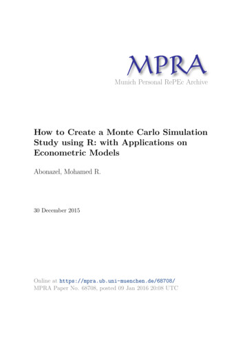
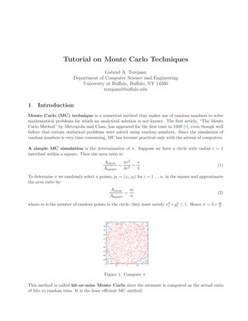
Tutorial on Monte Carlo TechniquesGabriel A. TerejanuDepartment of Computer Science and EngineeringUniversity at Buffalo, Buffalo, NY 14260terejanu@buffalo.edu1IntroductionMonte Carlo (MC) technique is a numerical method that makes use of random numbers to solvemathematical problems for which an analytical solution is not known. The first article, “The MonteCarlo Method” by Metropolis and Ulam, has appeared for the first time in 1949 [9], even though wellbefore that certain statistical problems were solved using random numbers. Since the simulation ofrandom numbers is very time consuming, MC has became practical only with the advent of computers.A simple MC simulation is the determination of π. Suppose we have a circle with radius r 1inscribed within a square. Then the area ratio is:Acircleπr 2π 2 Asquare4r4(1)To determine π we randomly select n points, pi (xi , yi ) for i 1 . . . n, in the square and approximatethe area ratio by:mAcircle Asquaren(2)where m is the number of random points in the circle, they must satisfy x2i yi2 1. Hence π 4 mn.10.80.60.40.20 0.2 0.4 0.6 0.8 1 1 0.500.51Figure 1: Compute πThis method is called hit-or-miss Monte Carlo since the estimate is computed as the actual ratioof hits to random tries. It is the least efficient MC method.
2Random VariablesThe “Monte Carlo” name is derived from the city, with the same name, in the Principality of Monaco,well known for its casinos. This was because the roulette wheel was the simplest mechanical devicefor generating random numbers [10].Even though “random variable” implies that one cannot predict its value, the distribution maywell be known. The distribution of a random variable gives the probability of a given value [7].The probability distribution of a discrete random variable is a list of probabilities associatedwith each of its possible values. It is also sometimes called the probability function or the probability mass function. (Valerie J. Easton and John H. McColl’s Statistics Glossary v1.1).A continuous random variable, x, takes any values in a certain interval (a, b). It is definedby probability density function (pdf ) p(x) and the given interval. The probability of xi falling inan arbitrary interval (a′ , b′ ) is given by:′′P{a x b } Zb′p(x)dx(3)a′The pdf has to satisfy the following two conditions:1. p(x) 0 for any x (a, b)Rb2. a p(x)dx 1The expected value or mean, the second moment and the variance or central second moment ofthe random variable are respectively defined by:E[x] µ Zbxp(x)dx(4)x2 p(x)dx(5)(x µ)2 p(x)dx E[x2 ] µ2(6)aE[x2 ] Zba22V ar[x] σ E[(x µ) ] Zabwhere σ is the standard deviation.Consider now two continuous random variables x and y. We say that x and y are statistically independent if the distribution of x does not depend on y and vice-versa. Hence the joint probabilitydensity function fxy (x, y) fx (x)fy (y).The covariance and the correlation of two random variables:Cov[x, y] E [(x E[x])(y E[y])] E[xy] E[x]E[y]Cov[x, y]Corr[x, y] pV ar[x]V ar[y]2(7)(8)
Note: If x and y are uncorrelated then their covariance and the correlation coefficient is zero, henceE[xy] E[x]E[y]. “Statistically independent random variables are always uncorrelated, but uncorrelated random variables can be dependent. Let x be uniformly distributed over [ 1, 1] and let y x2 .The two random variables are uncorrelated but are clearly not independent” [8].3Generate Random VariablesThe “Monte Carlo” name is derived from the city, with the same name, in the Principality of Monaco,well known for its casinos. This was because the roulette wheel was the simplest mechanical devicefor generating random numbers [10].“A sequence of truly random numbers is unpredictable and therefore unreproducible. Such a sequence can only be generated by a random physical process” [7]. Practically it is very difficult toconstruct such a physical generator, which has to be fast enough, and to connect it to a computer. Toovercome this problem one can use pseudo-random numbers, which are computed according to amathematical formulation, hence are reproducible and appear random to someone who does not knowthe algorithm [12].John von Neumann has constructed the first pseudorandom generator called mid-square method.Suppose we have a 4-digit number x1 0.9876. We square it, x21 0.97535376, obtaining this way a8-digit number. We obtain x2 by taking out the middle four digits, hence x2 0.5353. Now squarex2 and so on. Unfortunately, the algorithm tends to produce disproportionate frequency of smallnumbers [10].One popular algorithm is the multiplicative congruential method suggested by D.H. Lehmerin 1949. Given a modulus m, a multiplier a and a starting point x1 , the method generates successivepseudo-random numbers by the formula [7]:xi axi 1 M od(m)4(9)MC integrationLet f (x) be an arbitrary continuous function and y f (x) the new random variable. Then theexpected value and the variance of y:Z bf (x)p(x)dx(10)E[y] E[f (x)] aZ b(f (x) E[f (x)])2 p(x)dx(11)V ar[y] V ar[f (x)] aNote: E[f (x)] 6 f (E[x]).Our goal is to calculate the expectation of f (x) without computing the integral. This can be achievedby using a MC simulation.3
Crude Monte Carlo: A simple estimate of the integral (10) can Pbe obtained by generating n1samples xi q(x), for i 1 . . . n, and computing the estimate I n ni 1 f (xi ). To determine theaccuracy of method we first have to introduce two theorems.The law of large numbers implies that the average of a sequence of random variables, of a knowndistribution, converge to its expectation as the numbers of samples goes to infinity. Let us select nnumbers xi randomly with probability density p(x). Hence:n1XI f (xi ) E[f (x)] ni 1Zbf (x)p(x)dx(12)aIn the statistical context A(n) is a consistent estimator of B if “A(n) is said to converge to B asn goes to infinity if for any probability P [0 P 1], and any positive quantity δ, a k can be foundsuch that for all n k the probability that A(n) will be within δ of B is greater that P ” [7].The central limit theorem: the sum of a large number of independent random variables is approximately normally distributed. A sum of identical and independent distribution (i.i.d) randomvariables zi with mean µ an finite variance σ 2 :Pnzi nµi 1 N (0, 1) as n (13)σ nThe error of the MC method [2]:error I E[f (x)]n1Xf (xi ) E[f (x)]ni 1pPnV ar[f (x)]f (xi ) nE[f (x)]i 1 p nV ar[f (x)] npV ar[f (x)] N (0, 1) n(14)Mathematical properties [7]1. If the variance of f (x) is finite, the MC estimate is consistent2. The MC estimate is asymptotically unbiased3. The MC estimate is asymptotically normally distributed4. The standard deviation of the MC estimate is given by σ V ar[f (x)] nAlso note that the MC methods are immune to the curse of dimensionality. The accuracy of themethod can be improved by increasing the number of samples, n, but the convergence is very slow. Abetter way to improve the accuracy is to decrease the variance, V ar[f (x)]. This methods are calledvariance-reducing techniques.4
55.1Variance Reducing TechniquesStratified SamplingThis technique divides the full integration space into subspaces, for which a MC integration is performed. The final result is the sum of all partial results. We divide the integration domain R into kregions Ri for i 1 . . . k.E[f (x)] Zf (x)p(x)dx Rk ZXj 1f (x)p(x)dx(15)RjThe MC estimate of the expectation becomes:I njkXV ol(Rj ) Xnjj 1f (xi )(16)i 1where nj is the number of points used for MC integration on Rj , and V ol(Rj ) is the subdomain volume.The MC variance:σ2 kXV ol2 (Rj )j 1where V arRj [f (x)] nj1V ol(Rj )ZV arRj [f (x)]Rj1f (x) V ol(Rj )(17)Zf (x)p(x)dxRj!2p(x)dx(18)By selecting carefully the number of points this can lead to a lower variance compared with the crudeMC. If not it can perform worse than the crude MC.5.2Importance SamplingThe pdf under the integral, p(x), may not be the best pdf for MC integration. In this case we wantto use a different and simpler pdf q(x) from which we can draw the samples. q(x) is called theimportance density or the proposal distribution. Therefore we can write:ZE[y] E[f (x)] bf (x)p(x)dxbf (x)p(x)q(x)dxq(x)a f (x)p(x) Eq(x)Z (19)a(20)(21)By generating n samples xi q(x), for i 1 . . . n, the estimate becomes:nI n1X1 X f (xi )p(xi ) W (xi )f (xi )nq(xi )ni 1i 15(22)
i)Since the normalizing factor p(xi ) is not know,where W (xi ) p(xq(xi ) are the importance weights.Pwe have to normalize the weights such that ni 1 W (xi ) 1:n1 Pn1Xi 1 W (xi )f (xi )nP Wn (xi )f (xi )(23)I n1ni 1 W (xi )ni 1i)are the normalized importance weights. This estimate is biased butwhere Wn (xi ) P nW (xi 1 W (xi )the bias vanishes asymptotically as n [4].The variance of the importance sampler estimate is given by [4]: Z Ep2 [f (x)]1(f (x)p(x))2V arq [f (x)] dx nq(x)n(24)To reduce the variance q(x) should be chosen to match the shape of p(x) or f (x) p(x) [4].5.3Control VariatesSuppose that we have a function g(x) for which E[g(x)] is known. Let: h(x) f (x) c g(x) E[g(x)](25)where h(x) can have a smaller variance than f (x). Our estimate is given now by:n 1Xf (xi ) cg(xi ) cE[g(x)]I n(26)i 1The variance of h(x):V ar[h(x)] V ar[f (x)] c2 V ar[g(x)] 2cCov[f (x), g(x)](27)where Cov[f (x), g(x)] E [(f (x) E[f (x)])(g(x) E[g(x)])].We want to minimize the variance V ar[h(x)] with respect to c:dV ar[h(x)] 2cV ar[g(x)] 2Cov[f (x), g(x)]dc(28)By setting this to zero, the optimal value for c is then given by:c Cov[f (x), g(x)]V ar[g(x)](29)Then the variance V ar[h(x)] becomes:V ar[h(x)] V ar[f (x)] where Corr[f (x), g(x)] Cov 2 [f (x), g(x)] V ar[f (x)] 1 Corr 2 [f (x), g(x)])V ar[g(x)]Cov[f (x),g(x)] V ar[f (x)] V ar[g(x)](30)is the correlation coefficient. Hence the quality of theestimation depends on the correlation between f (x) and g(x).6
5.4Rejection Sampling (or Acceptance Rejection Sampling)Suppose that we know an upper bound for the underlying pdf p(x) and we use a proposal distributionq(x) as in importance sampling. So, there is c such that p(x) cq(x) [4].Algorithm 1 Rejection Sampling1: Select a uniform random variable u U(0, 1)2: Draw a sample x q(x)p(x)3: if u cq(x) then4:accept x5: else6:reject it and repeat the process7: end ifOne should carefully select the value for c. If it is too small the rejection rate will be low; if it is toobig the acceptance rate will be low.5.5Antithetic VariatesConsider that we have an even number of samples, 2n, drawn from p(x). One approach is to generatecorrelated samples to reduce the variance by cancellations in their sum. The estimate:2nI 1 Xf (xi )2n1ni 1nXi 1f (x2i 1 ) f (x2i )2n1Xg(x2i )n(31)(32)(33)i 1where g(x2i ) f (x2i 1 ) f (x2i ).2The variance V ar[g(x2i )]: f (x2i 1 ) f (x2i )V ar[g(x2i )] V ar2 1V ar[f (x2i 1 )] V ar[f (x2i )] 2Cov[f (x2i 1 ), f (x2i )] 4(34)(35)Variance analysis:1. If Cov[f (x2i 1 ), f (x2i )] 0 or f (x2i 1 ), f (x2i ) are independent then V ar[g(x2i )] 21 V ar[f (x2i 1 )],hence the variance of the estimator remains the same.2. If Cov[f (x2i 1 ), f (x2i )] 0 then the estimate is improved.3. If Cov[f (x2i 1 ), f (x2i )] 0 the actual performance is worse.7
5.6Partial averaging (or Rao-Blackwellization)The method is based on the idea that “one should carry out analytical computation as much as possible” [3]. So, if we can analytically compute the integral over a subspace, this yields the same expectedvalue but with a smaller variance.From the Law of Iterated Expectations we can compute the conditional expectation of f (x) for somesigma algebra F: E[f (x)] E E[f (x) F](36)From the Law of Total Variance: V ar[f (x)] V ar E[f (x) F] E V ar[f (x) F](37) Therefore V ar[f (x)] V ar E[f (x) F] . In practice we can factor f (x) such that some of the partsto be computed analytical and the rest can be solved by using Monte Carlo simulation. The methodcan be very problem dependent due to this factorization and sometimes may be more computationalexpensive than just simulating the entire system [3].6Markov Chain Monte CarloMCMC deals with generating samples from some complex probability distribution p(x) that is difficultto directly sample from. The approach is to use a sequence of samples {xk } from a Markov chain,such that the sequence converges on p(x) as k .In the following section only the case of discrete-time, continuous state space Markov process is discussed.6.1Markov chainA Markov process is a stochastic process that has the Markov property. A stochastic process hasthe Markov property if the conditional probability distribution of the future states given all the paststates depends only on the current state:p(xk 1 x0 , x1 . . . xk ) p(xk 1 xk )(38)A Markov chain is a sequence of random variables {xk } generated by a Markov processes. Thevalue of xk is called the state of the process at time k. The one step transition probabilitydensity (transition kernel) p(y x) is the probability density that the process moves from x to y.The transition kernel must satisfy:Zp(y x)dy 1(39)Definition: The Markov chain is said to be homogeneous/stationary if the transition kernels donot depend on the time.8
Define p(x) the total probability density of x, and p(x0 ) the initial probability density of x0 .The total probability density of y is given by the Chapman-Kolmogorov equation:Zp(y) p(y x)p(x)dx(40)Theorem: “If a Markov chain is ergodic, then there exists a unique steady state distribution πindependent of the initial state” [4].Zπ(y) p(y x)π(x)dx(41)Reversible condition (detailed balance property): Guarantees the invariance of π under thetransition kernel:p(x y)π(y) p(y x)π(x), x, y(42)“The unconditional probability of moving y to x is equal to the unconditional probability of movingx to y, where x and y are both generated from π(·)” [4].“In MCMC sampling framework the samples are generated by a homogeneous, reversible, ergodicMarkov chain with invariant distribution π” [4].6.2Metropolis-Hastings AlgorithmPublished in 1953 by Nicholas Metropolis and generalized in 1970 by W.K.Hastings, the algorithmdraws samples from the target density π(x), for which the normalizing factor might be unknown.RA Markov chain is generated with a proposal density (candidate target) q(y x), where q(y x)dx 1. The proposal density generates a value for y when the process is at x [5]. If q(y x) satisfies thereversible condition then our search for a transition kernel is over.Suppose, without loss of generality, that:q(y x)π(x) q(x y)π(y)(43)which means that the process moves from x to y much often than from y to x [5]. To reduce thenumber of moves from x to y one can introduce the probability of move, α(y x), such that thetransition kernel from x to y is given by:pM H (y x) q(y x)α(y x)(44)From (43) set α(x y) 1, because we need as many moves as we can get from y to x. To determineα(y x), one must require pM H (y x) to have the detailed balance property:pM H (y x)π(x) pM H (x y)π(y)(45)q(y x)α(y x)π(x) q(x y)α(x y)π(y) q(x y)π(y)9(46)
Thus the probability of move is given by: q(x y)π(y)α(y x) min,1q(y x)π(x)(47)Algorithm 2 Metropolis-Hasting1: Draw x0 from p(x0 )2: for i 0 to N do3:Generate y q(y xi )4:Generate u U(0, 1)5:if u α(y xi ) then6:xi 1 y7:else8:xi 1 xi9:end if10: end for11: return {xN b , xN b 1 , . . . xN }The number of steps, N , determines the algorithm performance. We need a good amount of steps,denoted N b, for the chain to approaches stationarity (burn-in period). Another important factor forthe efficiency is to have many samples or a high acceptance rate for the values of y. The draws areregarded as samples from π(x) only after the burn-in period N b [5].6.3Gibbs SamplingThe method was introduced by German and German in 1984 and named after the physicist J.W.Gibbs. The algorithm is a special case of Metropolis-Hastings for generating a sequence of samplesfrom a joint distribution p(x) hard to sample, of two or more random variables.Let x be a n-dimensional random vector: x [x1 , x2 , . . . xn ]T . The Gibbs sampler uses only univariate conditional distributions, where all of the random variables but one are assigned fixed values.Algorithm 3 Gibbs Sampling1: Draw x0 from p(x0 ), results : x0 [x01 , x02 , . . . x0n ]T2: for i 1 to N doi 1i 13:Draw xi1 p(x1 xi 12 , x3 , . . . xn )4:.i 1i 15:Draw xin p(xn xi 11 , x2 , . . . xn 1 )6:xi [xi1 , xi2 , . . . xin ]T7: end for8: return {xN b , xN b 1 , . . . xN }where N b denotes the burn-in period.10
“The Gibbs sampler is a nice solution to estimation of hierarchical or structured probabilistic model.Gibbs sampling can be viewed as a Metropolis method in which the proposal distribution is defined interms of the conditional distributions of the joint distribution and every proposal is always accepted”[4].7Sequential Monte CarloIn this section we focus our attention on sequential state estimation using sequential Monte Carlo(SMC). SMC is known also as bootstrap filtering, particle filtering, the condensation algorithm, interacting particle approximations and survival of the fittest [1].7.1Sequential Importance Sampling (SIS)Consider the following nonlinear system, described by the difference equation and the observationmodel:xk f(xk 1 , wk 1 )(48)zk h(xk , vk 1 )(49)Denote by Zk {zi 1 i k} the set of all observations up to time k, conditionally independentgiven the process with distribution p(zk xk ). Also, assume that the state sequence xk is an unobserved(hidden) Markov process with initial distribution p(x0 ) and transition distribution p(xk 1 xk ) [6].Our aim is to estimate recursively the posterior distribution p(xk Zk ) and expectations of the form[6]:ZE[f (xk , wk )] f (xk , wk )p(xk Zk )dxk(50)Suppose that we cannot sample from the posterior distribution and use an importance samplingapproach to sample from a proposal distribution q(xk Zk ). Hence:Zp(xk Zk )q(xk Zk )dxk(51)E[f (xk , wk )] f (xk , wk )q(xk Zk )Zp(Zk xk )p(xk )q(xk Zk )dxk(52) f (xk , wk )p(Zk )q(xk Zk )ZWk (xk ) f (xk , wk )q(xk Zk )dxk(53)p(Zk )k Zk )k xk )p(xk ) p(xwhere Wk (xk ) p(Zq(xq(xk Zk ) are the unnormalized importance weights. One can get rid ofk Zk )the unknown normalizing density p(Zk ) by deriving the expectation as:Rf (xk , wk )Wk (xk )q(xk Zk )dxk(54)E[f (xk , wk )] Rk Zk )p(Zk xk )p(xk ) q(xq(xk Zk ) dxk Eq [Wk (xk )f (xk , wk )]Eq [Wk (xk )]11(55)
By drawing N samples {xik } q(xk Zk ), i 1 . . . N , one can approximate the expectations:1 PNiii 1 Wk (xk )f (xk , wk )NE[f (xk , wk )] PN1ii 1 Wk (xk )N NXW̄k (xik )f (xik , wk )(56)(57)i 1where W̄k (xik ) Wk (xik )PNii 1 Wk (xk )are the normalized weights.Since it is very hard to find a good proposal distribution in a high dimensional space, one can sequentially construct it. Suppose we can factorize the proposal distribution:q(xk Zk ) q(xk xk 1 , Zk )q(xk 1 , Zk 1 )(58)The posterior distribution can be factorized as:p(zk xk )p(xk xk 1 )p(zk Zk 1 ) p(xk 1 Zk 1 )p(zk xk )p(xk xk 1 )p(xk Zk ) p(xk 1 Zk 1 )(59)(60)Hence we can recursively update the weights:Wk (xik ) p(xik Zk )q(xik Zk )(61)p(xik 1 Zk 1 )p(zk xik )p(xik xik 1 )q(xik xik 1 , Zk )q(xik 1 , Zk 1 ) Wk 1 (xik 1 )Algorithm 4 Sequential Importance Sampling1: Draw xik q(xk xik 1 , Zk ) for i 1 . . . N2:iCompute the importance weights Wki Wk 13:Normalize the importance weights W̄ki p(zk xik )p(xik xik 1 )q(xik xik 1 , Zk )(62)(63)p(zk xik )p(xik xik 1 )q(xik xik 1 ,Zk )WiPN k ii 1 WkDegeneracy problem: After a few iterations all but one particle will have negligible weights. Hencethe algorithms allots time to update a large number of weights with no effect in our sampling.Proposition (Kong et al. 1994): The unconditional variance (that is, when the observationsare regarded as random) of the importance ratios increases over time, where the importance ratiois given by:Wk (xik ) p(xik Zk )q(xik Zk )This problem can be overcome by adding a resampling strategy to SIS algorithm.12(64)
7.2Sequential Importance Resampling (SIR)The resampling step eliminates the samples with low importance weights and multiplies the ones withhigh importance weights. “Many of the ideas on resampling have stemmed from the work of Efron1982, Rubin 1988, and Smith and Gelfand 1992” [11].To detect the weights degeneracy (or sample impoverishment), one can use the effective samplesize Nef f given by [4]:Nef f N1 V arq [W̄k (xk )]NEq [W̄k (x2k )](65)(66)An estimate of the effective sample size:N̂ef f NPNi 2i 1 (W̄k )(67)If N̂ef f is less than an given threshold then run the resampling step.One approach is to draw N particles from the current set of particles with probabilities proportional to their weights and set the new weights to N1 . This can be done by generating a new setof indices from a CDF that maps the random measure {xik , W̄ki } into an equally weighted randommeasure {xjk , N1 } [11].Figure 2: Resampling process [11]13
Algorithm 5 Resampling Algorithm1: Initialize CDF : c1 02: Construct CDF : ci ci 1 W̄ki , for all i 1 . . . N3: for j 1 to N do4:Sampling index: u U(0, 1)5:Resampling index: i CDF 1 (u)N6:Assign sample: x̃jk xik7:Assign weight: W̄kj N18: end forjj9: return the new set {x̃k , W̄k }where CDF 1 (·) is the inverse of the CDF (·) function.This step reduces the sample impoverishment effect but introduces new practical problems: it limitsthe opportunity to have a parallel algorithm, particles with high weights are statistically selected manytimes and leads to a loss of diversity among the particles [1].References[1] M.S. Arulampalam, S. Maskell, N. Gordon, and T. Clapp. A Tutorial on Particle Filters forOnline Nonlinear/Non-Gaussian Bayesian Tracking. IEEE Trans. on Signal Processing, 50, 2002.[2] Paul J. Atzberger.Strategies for Improving the Efficiency of Monte-Carlo Methods.http://www.cims.nyu.edu/ paulatz/class finance/improvingMonteCarloMethods.pdf.[3] K.R. Beevers. Monte Carlo integration. Lecture Notes for CSCI-6971, 2006.[4] Zhe Chen. Bayesian Filtering: From Kalman Filters to Particle Filters, and Beyond. Manuscript.[5] S. Chib and E. Greenberg. Understanding the Metropolis-Hastings algorithm. The AmericanStatistician, 1995.[6] A. Doucet, S. Godsill, and C. Andrieu. On Sequential Monte Carlo Sampling Methods for BayesianFiltering. Technical report, Signal Processing Group, Department of Engineering, University ofCambridge, UK.[7] F. James. Monte Carlo Theory and Practice. Rep. Prog. Phys., 43:1147–1188, 1980.[8] D. Johnson. Jointly Distributed Random Variables. http://cnx.org/content/m11248/latest/,2005.[9] N. C. Metropolis and S. M. Ulam. The Monte-Carlo Method. J. Amer. Stat. Assoc., 44:335–341,1949.[10] Ilya M. Sobol’. A Primer for the Monte Carlo Method. CRC Press, 1994.[11] Rudolph van der Merwe, Nando de Freitas, Arnaud Doucet, and Eric Wan. The unscented particelfilter. In Advances in Neural Information Processing Systems 13, Nov 2001.14
[12] S. Weinzierl. Introduction to Monte Carlo Methods. Technical report, NIKHEF Theory Group,2000.15
Tutorial on Monte Carlo Techniques Gabriel A. Terejanu Department of Computer Science and Engineering University at Buffalo, Buffalo, NY 14260 terejanu@buffalo.edu 1 Introduction Monte Carlo (MC) technique is a numerical method that makes use of random numbers to solve mathematical problems for which an analytical solution is not known.