Transcription
18PROC. OF THE 14th PYTHON IN SCIENCE CONF. (SCIPY 2015)librosa: Audio and Music Signal Analysis in PythonBrian McFee¶§ , Colin Raffel‡ , Dawen Liang‡ , Daniel P.W. Ellis‡ , Matt McVicar , Eric Battenbergk , Oriol Nieto§https://www.youtube.com/watch?v MhOdbtPhbLUFAbstract—This document describes version 0.4.0 of librosa: a Python package for audio and music signal processing. At a high level, librosa providesimplementations of a variety of common functions used throughout the field ofmusic information retrieval. In this document, a brief overview of the library’sfunctionality is provided, along with explanations of the design goals, softwaredevelopment practices, and notational conventions.Index Terms—audio, music, signal processingIntroductionThe emerging research field of music information retrieval (MIR)broadly covers topics at the intersection of musicology, digitalsignal processing, machine learning, information retrieval, andlibrary science. Although the field is relatively young—the firstinternational symposium on music information retrieval (ISMIR)1was held in October of 2000—it is rapidly developing, thanks inpart to the proliferation and practical scientific needs of digitalmusic services, such as iTunes, Pandora, and Spotify. While thepreponderance of MIR research has been conducted with customtools and scripts developed by researchers in a variety of languagessuch as MATLAB or C , the stability, scalability, and ease of usethese tools has often left much to be desired.In recent years, interest has grown within the MIR communityin using (scientific) Python as a viable alternative. This hasbeen driven by a confluence of several factors, including theavailability of high-quality machine learning libraries such asscikit-learn [Pedregosa11] and tools based on Theano[Bergstra11], as well as Python’s vast catalog of packages fordealing with text data and web services. However, the adoption ofPython has been slowed by the absence of a stable core library thatprovides the basic routines upon which many MIR applicationsare built. To remedy this situation, we have developed librosa:2 aPython package for audio and music signal processing.3 In doingso, we hope to both ease the transition of MIR researchers intoPython (and modern software development practices), and also* Corresponding author: brian.mcfee@nyu.edu¶ Center for Data Science, New York University§ Music and Audio Research Laboratory, New York University‡ LabROSA, Columbia University** Department of Engineering Mathematics, University of Bristol Silicon Valley AI Lab, Baidu, Inc.Copyright 2015 Brian McFee et al. This is an open-access article distributedunder the terms of the Creative Commons Attribution License, which permitsunrestricted use, distribution, and reproduction in any medium, provided theoriginal author and source are credited.to make core MIR techniques readily available to the broadercommunity of scientists and Python programmers.Design principlesIn designing librosa, we have prioritized a few key concepts. First,we strive for a low barrier to entry for researchers familiar withMATLAB. In particular, we opted for a relatively flat packagelayout, and following scipy [Jones01] rely upon numpy datatypes and functions [VanDerWalt11], rather than abstract classhierarchies.Second, we expended considerable effort in standardizinginterfaces, variable names, and (default) parameter settings acrossthe various analysis functions. This task was complicated by thefact that reference implementations from which our implementations are derived come from various authors, and are oftendesigned as one-off scripts rather than proper library functionswith well-defined interfaces.Third, wherever possible, we retain backwards compatibilityagainst existing reference implementations. This is achieved viaregression testing for numerical equivalence of outputs. All testsare implemented in the nose framework.4Fourth, because MIR is a rapidly evolving field, we recognizethat the exact implementations provided by librosa may notrepresent the state of the art for any particular task. Consequently,functions are designed to be modular, allowing practitioners toprovide their own functions when appropriate, e.g., a custom onsetstrength estimate may be provided to the beat tracker as a functionargument. This allows researchers to leverage existing libraryfunctions while experimenting with improvements to specificcomponents. Although this seems simple and obvious, from apractical standpoint the monolithic designs and lack of interoperability between different research codebases have historicallymade this difficult.Finally, we strive for readable code, thorough documentation and exhaustive testing. All development is conducted onGitHub. We apply modern software development practices, suchas continuous integration testing (via Travis5 ) and coverage (viaCoveralls6 ). All functions are implemented in pure Python, thoroughly documented using Sphinx, and include example codedemonstrating usage. The implementation mostly complies with1. http://ismir.net2. https://github.com/bmcfee/librosa3. The name librosa is borrowed from LabROSA : the LABoratory for theRecognition and Organization of Speech and Audio at Columbia University,where the initial development of librosa took place.4. https://nose.readthedocs.org/en/latest/
LIBROSA: AUDIO AND MUSIC SIGNAL ANALYSIS IN PYTHONPEP-8 recommendations, with a small set of exceptions for variable names that make the code more concise without sacrificingclarity: e.g., y and sr are preferred over more verbose names suchas audio buffer and sampling rate.ConventionsIn general, librosa’s functions tend to expose all relevant parameters to the caller. While this provides a great deal of flexibility toexpert users, it can be overwhelming to novice users who simplyneed a consistent interface to process audio files. To satisfy bothneeds, we define a set of general conventions and standardizeddefault parameter values shared across many functions.An audio signal is represented as a one-dimensional numpyarray, denoted as y throughout librosa. Typically the signal y isaccompanied by the sampling rate (denoted sr) which denotesthe frequency (in Hz) at which values of y are sampled. Theduration of a signal can then be computed by dividing the numberof samples by the sampling rate: duration seconds float(len(y)) / srBy default, when loading stereo audio files, thelibrosa.load() function downmixes to mono by averagingleft- and right-channels, and then resamples the monophonicsignal to the default rate sr 22050 Hz.Most audio analysis methods operate not at the native samplingrate of the signal, but over small frames of the signal which arespaced by a hop length (in samples). The default frame and hoplengths are set to 2048 and 512 samples, respectively. At thedefault sampling rate of 22050 Hz, this corresponds to overlappingframes of approximately 93ms spaced by 23ms. Frames arecentered by default, so frame index t corresponds to the slice:y[(t * hop length - frame length / 2):(t * hop length frame length / 2)],where boundary conditions are handled by reflection-padding theinput signal y. Unless otherwise specified, all sliding-windowanalyses use Hann windows by default. For analyses that do notuse fixed-width frames (such as the constant-Q transform), thedefault hop length of 512 is retained to facilitate alignment ofresults.The majority of feature analyses implemented by librosa produce two-dimensional outputs stored as numpy.ndarray, e.g.,S[f, t] might contain the energy within a particular frequencyband f at frame index t. We follow the convention that the finaldimension provides the index over time, e.g., S[:, 0], S[:,1] access features at the first and second frames. Feature arraysare organized column-major (Fortran style) in memory, so thatcommon access patterns benefit from cache locality.By default, all pitch-based analyses are assumed to be relativeto a 12-bin equal-tempered chromatic scale with a referencetuning of A440 440.0 Hz. Pitch and pitch-class analysesare arranged such that the 0th bin corresponds to C for pitch classor C1 (32.7 Hz) for absolute pitch measurements.Package organizationIn this section, we give a brief overview of the structure of the librosa software package. This overview is intended to be superficialand cover only the most commonly used functionality. A completeAPI reference can be found at https://bmcfee.github.io/librosa.5. https://travis-ci.org6. https://coveralls.io19Core functionalityThe librosa.core submodule includes a range of commonlyused functions. Broadly, core functionality falls into four categories: audio and time-series operations, spectrogram calculation,time and frequency conversion, and pitch operations. For convenience, all functions within the core submodule are aliased at thetop level of the package hierarchy, e.g., librosa.core.loadis aliased to librosa.load.Audio and time-series operations include functionssuch as: reading audio from disk via the audioreadpackage7 (core.load), resampling a signal at a desiredrate (core.resample), stereo to mono conversion(core.to mono), time-domain bounded auto-correlation(core.autocorrelate), and zero-crossing detection(core.zero crossings).Spectrogram operations include the short-time Fourier transform (stft), inverse STFT (istft), and instantaneous frequency spectrogram (ifgram) [Abe95], which provide muchof the core functionality for down-stream feature analysis. Additionally, an efficient constant-Q transform (cqt) implementation based upon the recursive down-sampling method of Schoerkhuber and Klapuri [Schoerkhuber10] is provided, which produces logarithmically-spaced frequency representations suitablefor pitch-based signal analysis. Finally, logamplitude provides a flexible and robust implementation of log-amplitude scaling, which can be used to avoid numerical underflow and set anadaptive noise floor when converting from linear amplitude.Because data may be represented in a variety of time orfrequency units, we provide a comprehensive set of conveniencefunctions to map between different time representations: seconds,frames, or samples; and frequency representations: hertz, constantQ basis index, Fourier basis index, Mel basis index, MIDI notenumber, or note in scientific pitch notation.Finally, the core submodule provides functionality to estimatethe dominant frequency of STFT bins via parabolic interpolation(piptrack) [Smith11], and estimation of tuning deviation (incents) from the reference A440. These functions allow pitch-basedanalyses (e.g., cqt) to dynamically adapt filter banks to match theglobal tuning offset of a particular audio signal.Spectral featuresSpectral representations—the distributions of energy over aset of frequencies—form the basis of many analysis techniques in MIR and digital signal processing in general. Thelibrosa.feature module implements a variety of spectralrepresentations, most of which are based upon the short-timeFourier transform.The Mel frequency scale is commonly used to represent audio signals, as it provides a rough model of human frequency perception [Stevens37]. Both a Mel-scale spectrogram (librosa.feature.melspectrogram) and thecommonly used Mel-frequency Cepstral Coefficients (MFCC)(librosa.feature.mfcc) are provided. By default, Melscales are defined to match the implementation provided bySlaney’s auditory toolbox [Slaney98], but they can be made tomatch the Hidden Markov Model Toolkit (HTK) by setting theflag htk True [Young97].While Mel-scaled representations are commonly used to capture timbral aspects of music, they provide poor resolution of7. https://github.com/sampsyo/audioread
20PROC. OF THE 14th PYTHON IN SCIENCE CONF. (SCIPY 2015)11025STFT log power8268Hz55122756010453Mel spectrogram log powerHz44621905799TonnetzPitch .86s30.72s33.58s36.44s39.30s42.16s0 dB-6 dB-12 dB-18 dB-24 dB-30 dB-36 dB-42 dB-48 dB-54 dB-60 dB0 dB-6 dB-12 dB-18 dB-24 dB-30 dB-36 dB-42 dB-48 dB-54 dB-60 50.000.150.300.4545.02sFig. 1: First: the short-time Fourier transform of ponding Mel spectrogram, using 128 Mel responding chromagram (librosa.feature.chroma cqt).Fourth: the Tonnetz features (librosa.feature.tonnetz).pitches and pitch classes. Pitch class (or chroma) representationsare often used to encode harmony while suppressing variationsin octave height, loudness, or timbre. Two flexible chroma implementations are provided: one uses a fixed-window STFT analysis(chroma stft)8 and the other uses variable-window constantQ transform analysis (chroma cqt). An alternative representation of pitch and harmony can be obtained by the tonnetzfunction, which estimates tonal centroids as coordinates in asix-dimensional interval space using the method of Harte etal. [Harte06]. Figure 1 illustrates the difference between STFT,Mel spectrogram, chromagram, and Tonnetz representations, asconstructed by the following code fragment:9and spectral contrast [Jiang02].10Finally, the feature submodule provides a few functionsto implement common transformations of time-series features inMIR. This includes delta, which provides a smoothed estimateof the time derivative; stack memory, which concatenates aninput feature array with time-lagged copies of itself (effectivelysimulating feature n-grams); and sync, which applies a usersupplied aggregation function (e.g., numpy.mean or median)across specified column intervals.DisplayThe display module provides simple interfaces to visuallyrender audio data through matplotlib [Hunter07]. The firstfunction, display.waveplot simply renders the amplitudeenvelope of an audio signal y using matplotlib’s fill betweenfunction. For efficiency purposes, the signal is dynamically downsampled. Mono signals are rendered symmetrically about thehorizontal axis; stereo signals are rendered with the left-channel’samplitude above the axis and the right-channel’s below. An example of waveplot is depicted in Figure 2 (top).The second function, display.specshow wraps matplotlib’s imshow function with default settings (origin andaspect) adapted to the expected defaults for visualizing spectrograms. Additionally, specshow dynamically selects appropriatecolormaps (binary, sequential, or diverging) from the data typeand range.11 Finally, specshow provides a variety of acoustically relevant axis labeling and scaling parameters. Examples ofspecshow output are displayed in Figures 1 and 2 (middle).Onsets, tempo, and beatsIn addition to Mel and chroma features, thefeature submodule provides a number of spectralstatistic representations, including spectral centroid,spectral bandwidth, spectral rolloff [Klapuri07],While the spectral feature representations described above capturefrequency information, time information is equally important formany applications in MIR. For instance, it can be beneficial toanalyze signals indexed by note or beat events, rather than absolutetime. The onset and beat submodules implement functions toestimate various aspects of timing in music.More specifically, the onset module provides twofunctions: onset strength and onset detect. Theonset strength function calculates a thresholded spectralflux operation over a spectrogram, and returns a one-dimensionalarray representing the amount of increasing spectral energy at eachframe. This is illustrated as the blue curve in the bottom panelof Figure 2. The onset detect function, on the other hand,selects peak positions from the onset strength curve followingthe heuristic described by Boeck et al. [Boeck12]. The output ofonset detect is depicted as red circles in the bottom panel ofFigure 2.The beat module provides functions to estimate the globaltempo and positions of beat events from the onset strength function, using the method of Ellis [Ellis07]. More specifically, thebeat tracker first estimates the tempo, which is then used to set thetarget spacing between peaks in an onset strength function. Theoutput of the beat tracker is displayed as the dashed green lines inFigure 2 (bottom).8. chroma stft is based upon the reference implementation provided yn/9. logamplitude. We refer readers to the accompanyingIPython notebook for the full source code to recontsruct figures.10. spectral * functions are derived from MATLAB reference implementations provided by the METLab at Drexel University. http://music.ece.drexel.edu/11. If the seaborn package [Waskom14] is available, its version ofcubehelix is used for sequential data. . . . filename librosa.util.example audio file()y, sr librosa.load(filename,offset 25.0,duration 20.0)spectrogram np.abs(librosa.stft(y))melspec librosa.feature.melspectrogram(y y,sr sr)chroma librosa.feature.chroma cqt(y y,sr sr)tonnetz librosa.feature.tonnetz(y y, sr sr)
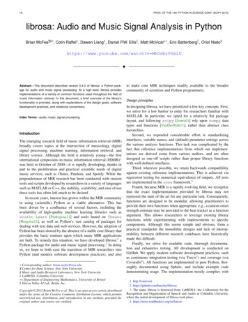
LIBROSA: AUDIO AND MUSIC SIGNAL ANALYSIS IN PYTHON21y (mono signal)11025STFT log powerHz219610984520Onset strengthDetected note onsetsDetected 06sFig. 2: Top: a waveform plot for a 20-second audio clip y, generated by librosa.display.waveplot. Middle: the log-power short-timeFourier transform (STFT) spectrum for y plotted on a logarithmic frequency scale, generated by librosa.display.specshow. Bottom:the onset strength function (librosa.onset.onset strength), detected onset events (librosa.onset.onset detect), anddetected beat events (librosa.beat.beat track) for y.Tying this all together, the tempo and beat positions foran input signal can be easily calculated by the following codefragment: y, sr librosa.load(FILENAME) tempo, frames librosa.beat.beat track(y y,.sr sr) beat times librosa.frames to time(frames,.sr sr)Any of the default parameters and analyses may be overridden.For example, if the user has calculated an onset strength envelopeby some other means, it can be provided to the beat tracker asfollows: oenv some other onset function(y, sr) librosa.beat.beat track(onset envelope oenv)All detection functions (beat and onset) return events as frameindices, rather than absolute timing. The downside of this is thatit is left to the user to convert frame indices back to absolutetime. However, in our opinion, this is outweighed by two practical benefits: it simplifies the implementations, and it makesthe results directly accessible to frame-indexed functions such aslibrosa.feature.sync.First, there are functions to calculate and ent.recurrence matrix constructs a binary knearest-neighbor similarity matrix from a given feature arrayand a user-specified distance function. As displayed in Figure 3(left), repeating sequences often appear as diagonal bands in therecurrence plot, which can be used to detect musical structure. Itis sometimes more convenient to operate in time-lag coordinates,rather than time-time, which transforms diagonal structures intomore easily detectable horizontal structures (Figure 3, right)[Serra12]. This is facilitated by the recurrence to lag (andlag to recurrence) functions.Second, temporally constrained clustering can be used todetect feature change-points without relying upon repetition. Thisis implemented in librosa by the segment.agglomerativefunction, which uses scikit-learn’s implementation ofWard’s agglomerative clustering method [Ward63] to partition the input into a user-defined number of contiguous components. In practice, a user can override thedefault clustering parameters by providing an existingsklearn.cluster.AgglomerativeClustering objectas an argument to segment.agglomerative().DecompositionsStructural analysisOnsets and beats provide relatively low-level timing cues formusic signal processing. Higher-level analyses attempt to detectlarger structure in music, e.g., at the level of bars or functionalcomponents such as verse and chorus. While this is an active areaof research that has seen rapid progress in recent years, there aresome useful features common to many approaches. The segmentsubmodule contains a few useful functions to facilitate structuralanalysis in music, falling broadly into two categories.Many applications in MIR operate upon latent factor representations, or other decompositions of spectrograms. For example,it is common to apply non-negative matrix factorization (NMF)[Lee99] to magnitude spectra, and analyze the statistics of theresulting time-varying activation functions, rather than the rawobservations.The decompose module provides a simple interface to factorspectrograms (or general feature arrays) into components andactivations:
22PROC. OF THE 14th PYTHON IN SCIENCE CONF. (SCIPY 2015)45.02s0.00sRecurrence plotLag 9.98s27.86s25.00s25.00s 27.86s 30.72s 33.58s 36.44s 39.30s 42.16s 45.02s0.00s25.00s 27.86s 30.72s 33.58s 36.44s 39.30s 42.16s 45.02sFig. 3: Left: the recurrence plot derived from the chroma features displayed in Figure 1. Right: the corresponding time-lag plot.harmonicpercussiveFor instance, rather than writing D librosa.stft(y) Dh, Dp librosa.decompose.hpss(D) y harmonic librosa.istft(Dh)one may simply write10453Harmonic mel spectrogramHz4462 y harmonic librosa.effects.harmonic(y)1905799010453Percussive mel spectrogramHz44621905Output799025.00sConvenience functions are provided for HPSS (retaining theharmonic, percussive, or both components), time-stretching andpitch-shifting. Although these functions provide no additionalfunctionality, their inclusion results in simpler, more readableapplication . 4: Top: the separated harmonic and percussive waveforms.Middle: the Mel spectrogram of the harmonic component. Bottom:the Mel spectrogram of the percussive component. comps, acts librosa.decompose.decompose(S)By default, the decompose() function constructsa scikit-learn NMF object, and applies itsfit transform() method to the transpose of S. Theresulting basis components and activations are accordinglytransposed, so that comps.dot(acts) approximates S. If theuser wishes to apply some other decomposition technique, anyobject fitting the sklearn.decomposition interface may besubstituted: T SomeDecomposer() librosa.decompose.decompose(S, transformer T)The output module includes utility functions to save theresults of audio analysis to disk. Most often, this takes theform of annotated instantaneous event timings or time intervals,which are saved in plain text (comma- or tab-separated values)via output.times csv and output.annotation, respectively. These functions are somewhat redundant with alternativefunctions for text output (e.g., numpy.savetxt), but providesanity checks for length agreement and semantic validation oftime intervals. The resulting outputs are designed to work withother common MIR tools, such as mir eval [Raffel14] andsonic-visualiser [Cannam10].The output module also provides the write wavfunction for saving audio in .wav format. The write wavsimply wraps the built-in scipy wav-file writer(scipy.io.wavfile.write) with validation and optionalnormalization, thus ensuring that the resulting audio files arewell-formed.CachingIn addition to general-purpose matrix decomposition techniques, librosa also implements the harmonic-percussive sourceseparation (HPSS) method of Fitzgerald [Fitzgerald10] asdecompose.hpss. This technique is commonly used in MIRto suppress transients when analyzing pitch content, or suppressstationary signals when detecting onsets or other rhythmic elements. An example application of HPSS is illustrated in Figure4.MIR applications typically require computing a variety of features(e.g., MFCCs, chroma, beat timings, etc) from each audio signalin a collection. Assuming the application programmer is contentwith default parameters, the simplest way to achieve this is to calleach function using audio time-series input, e.g.:EffectsHowever, because there are shared computations between thedifferent functions—mfcc and beat track both compute logscaled Mel spectrograms, for example—this results in redundantThe effects module provides convenience functions for applying spectrogram-based transformations to time-domain signals. mfcc librosa.feature.mfcc(y y, sr sr) tempo, beats librosa.beat.beat track(y y,.sr sr)
LIBROSA: AUDIO AND MUSIC SIGNAL ANALYSIS IN PYTHON(and inefficient) computation. A more efficient implementation ofthe above example would factor out the redundant features: lms am(y y,.sr sr)) mfcc librosa.feature.mfcc(S lms) tempo, beats librosa.beat.beat track(S lms,.sr sr)Although it is more computationally efficient, the above exampleis less concise, and it requires more knowledge of the implementations on behalf of the application programmer. More generally,nearly all functions in librosa eventually depend upon STFTcalculation, but it is rare that the application programmer willneed the STFT matrix as an end-result.One approach to eliminate redundant computation is to decompose the various functions into blocks which can be arranged ina computation graph, as is done in Essentia [Bogdanov13]. However, this approach necessarily constrains the function interfaces,and may become unwieldy for common, simple applications.Instead, librosa takes a lazy approach to eliminating redundancy via output caching. Caching is implemented through anextension of the Memory class from the joblib package12 ,which provides disk-backed memoization of function outputs.The cache object (librosa.cache) operates as a decorator onall non-trivial computations. This way, a user can write simpleapplication code (i.e., the first example above) while transparentlyeliminating redundancies and achieving speed comparable to themore advanced implementation (the second example).The cache object is disabled by default, but can be activatedby setting the environment variable LIBROSA CACHE DIR priorto importing the package. Because the Memory object does notimplement a cache eviction policy (as of version 0.8.4), it isrecommended that users purge the cache after processing eachaudio file to prevent the cache from filling all available diskspace13 . We note that this can potentially introduce race conditionsin multi-processing environments (i.e., parallel batch processing ofa corpus), so care must be taken when scheduling cache purges.Parameter tuningSome of librosa’s functions have parameters that require somedegree of tuning to optimize performance. In particular, theperformance of the beat tracker and onset detection functions canvary substantially with small changes in certain key parameters.After standardizing certain default parameters—sampling rate,frame length, and hop length—across all functions, we optimizedthe beat tracker settings using the parameter grid given in Table1. To select the best-performing configuration, we evaluated theperformance on a data set comprised of the Isophonics Beatlescorpus14 and the SMC Dataset2 [Holzapfel12] beat annotations.Each configuration was evaluated using mir eval [Raffel14],and the configuration was chosen to maximize the Correct MetricLevel (Total) metric [Davies14].Similarly, the onset detection parameters (listed in Table 2)were selected to optimize the F1-score on the Johannes KeplerUniversity onset database.1512. https://github.com/joblib/joblib13. The cache can be purged by calling librosa.cache.clear().14. s15. https://github.com/CPJKU/onset db23ParameterDescriptionValuesfmaxn melsaggregateMaximum frequency value (Hz)Number of Mel bandsSpectral flux aggregation functionac sizeMaximum lag for onset autocorrelation (s)Deviation of tempo estimatesfrom 120.0 BPMPenalty for deviation from estimated tempo8000, 1102532, 64, 128np.mean,np.median2, 4, 8std bpmtightness0.5, 1.0, 2.050, 100, 400TABLE 1: The parameter grid for beat tracking optimization. Thebest configuration is indicated in bold.ParameterDescriptionValuesfmaxMaximum frequency value(Hz)Number of Mel bandsSpectral flux aggregationfunctionPeak picking threshold8000, 11025n melsaggregatedelta32, 64, 128np.mean,np.median0.0--0.10 (0.07)TABLE 2: The parameter grid for onest detection optimization. Thebest configuration is indicated in bold.We note that the "optimal" default parameter settings aremerely estimates, and depend upon the datasets over which theyare selected. The parameter settings are therefore subject to changein the future as larger reference collections become available. Theoptimization framework has been factored out into a separaterepository, which may in subsequent versions grow to includeadditional parameters.16ConclusionThis document provides a brief summary of the design considerations and functionality of librosa. More detailed examples,notebooks, and documentation can be found in our developmentrepository and project website. The project is under active development, and our roadmap for future work includes efficiencyimprovements and enhanced functionality of audio coding and filesystem interactions.Citing librosaWe request that when using librosa in academic work, authors citethe Zenodo reference [McFee15]. For references to the design ofthe library, citation of the present document is appropriate.AcknowledgementsBM acknowledges support from the Moore-Sloan Data ScienceEnvironment at NYU. Additional support was provided by NSFgrant IIS-1117015.R EFERENCES[Pedregosa11]Pedregosa, Fabian, Gaël Varoquaux, Alexandre Gramfort,Vincent Michel, Bertrand Thirion, Olivier Grisel, MathieuBlondel et al. Scikit-learn: Machine learning in Python.The Journal of Machine Learning Re
signal processing, machine learning, information retrieval, and library science. Although the field is relatively young—the first international symposium on music information retrieval (ISMIR)1 was held in October of 2000—it is rapidly developing, thanks in part to the proliferation and practical scientific needs of digital