Transcription
Two-Way Repeated Measures ANOVAA repeated measures test is what you use when the same participants take part in all of theconditions of an experiment.This kind of analysis is similar to a repeated-measures (or paired samples) t-test, in that theyare both tests which are used to analyse data collected from a within participants designstudy. However, while the t-test limits you to situations where you only have oneindependent variable with two levels, a repeated measures ANOVA can be done when youhave more than two conditions, and/or more than one independent variable.In this tutorial we will consider an example where we have two independent variables andone dependent variable.Worked ExampleLet’s consider a fictional study designed to investigate how we mentally represent concepts.Imagine that we want to explore whether the way we think about specific objects (orconcepts) mirrors what we actually experience in real life, or whether these conceptrepresentations are independent of reality.For example, when we think of an object (e.g. a car), do we always think about it in thesame way? If concepts had no bearing on the real-world you might expect this to be thecase, as the underlying concept would always be the same. In contrast, just as changes incontext and perspective can alter how we see an object in the real world, do such changesalso affect our mental representations? If so, this would suggest concepts are representedas ‘perceptual simulations’ of the real world.To investigate this, participants were asked to read sentences (one at a time) that appearedon a computer screen. Each sentence placed them in different positions relative to anobject; for example, either inside (‘you are driving a car’) or outside (‘you are fuelling a car’)an object.Immediately after each sentence, participants saw a probe word that was either part of thatobject or not. To test the effect of functional perspective on mental representations, partsfrom two different locations were used: inside parts (e.g. a steering wheel) and outsideparts (e.g. a tyre).Participants had to verify, as quickly as possible, whether or not the part presentedbelonged to the object by pressing a key on the computer. Correct Response Times(measured in milliseconds) were taken as the Dependent Variable.
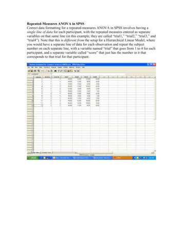
In this example, the experiment used a 2 x 2 repeated-measures design.The two independent variables were Functional Perspective andPart Location: Functional Perspective related to the position participants took in relation the theobject being imagined. It had two levels: Inside and Outside, depending on wherethe sentence they read had placed them. Part Type also had two levels, which were also Inside and Outside: depending onwhere the part named in the probe word was located on the target object.All participants took part in all of the conditions.This is what the data collected should look like in SPSS (and can be found in the SPSS file‘Week 4 Concepts Data.sav’):
As a general rule in SPSS, each row in the spreadsheet should contain all of the dataprovided by one participant.In a repeated measures design, this means that separate columns are needed to representeach of the conditions of the experiment. Please note that this differs from independenttests where the IVs are coded in separate columns and data for the different experimentalconditions is provided by separate individuals.In this example, we have two IVs, each with two levels. This means that each participanttakes part in four (2x2) conditions:1.2.3.4.Part Inside Inside Functional PerspectivePart Inside Outside Functional PerspectivePart Outside Inside Functional PerspectivePart Outside Outside Functional PerspectiveThe different columns in SPSS display the following data: ID No: This just refers to the ID number assigned to the participants. We usenumbers as identifiers instead of participant names, as this allows us to collect datawhile keeping the participants anonymous. PI FPI: This column displays each participant's mean reaction time in milliseconds(ms) to the inside part words (PI) when taking an inside functional perspective (FPI). PI FPO: This column displays each participant's mean reaction time to the insidepart words (PI) when taking an outside functional perspective (FPO). PO FPI: This column displays each participant's mean reaction time in milliseconds(ms) to the outside part words (PO) when taking an inside functional perspective(FPI). PO FPO: This column displays each participant's mean reaction time to the outsidepart words (PO) when taking an outside functional perspective (FPO).The Two-Way Repeated-Measures ANOVA compares the scores in the different conditionsacross both of the variables, as well as examining the interaction between them.In this case, we want to compare participant’s part verification time (measured inmilliseconds) for the two functional perspectives, the two part locations, and we want tolook at the interaction between these variables.
To start the analysis, begin by CLICKING on the Analyze menu, select the General LinearModel option, and then the Repeated Measures. sub-option.The “Repeated Measures Define Factor(s)” box should now appear. This is where we tellSPSS what our different IVs are, and how many levels they have. SPSS doesn’t mind whatnames we give the variables, but it’s probably a good idea to give them sensible nameswhich we can interpret easily when we look at the output. In this case, let’s name ourvariables Part Location (the underscore is used to separate the words, as SPSS doesn't likespaces in variable names) and Perspective.We can define our first variable by typing the name (Part Location) into the Within-SubjectFactor Name box, and entering the number of levels (2) into the Number of Levels box:CLICK on Add to add this variable to the analysis.
Next, we need to define the second independent variable in the same way.Again, CLICK on Add to add this variable to the analysis. And once you have finished definingyour IVs, CLICK on the Define button to continue with the analysis.This opens up the Repeated Measures dialog box. We now have to us this to tell SPSS theway our variable conditions fit into the ANOVA.
At the top of the Within-Subjects Variables box SPSS tells you that there are two factors tobe analyzed (the ones we have just named): Part Location and Perspective.In the box itself, there are a series of question marks with bracketed numbers. Thesenumbers represent the levels of our IVs. In this example, there are two IVs so there are alsotwo numbers in each of the brackets. The first number refers to the levels of the firstvariable we defined (Part Location), while the second refers to Perspective.Our task is to replace the question marks with the names of the conditions that match thevariable level codes.For example, the first line (1,1) means that we have to move across the condition thatcontains data for the first level of Part Loctaion (in this case: inside) and the first level ofPerspective (which is also 'inside'). So we have to CLICK on the condition that matches thisand move it across to the Within-Subjects Variables box by CLICKING on the arrow button.We then need to do the same for the following three conditions in the list.For example, the next position we want to fill is labelled (1,2), which means we want thecondition that contains data for the first level of Part Location (again, this is 'inside') and thesecond level of Perspective (i.e. outside). So we need to SELCET the matching condition andmove it across to the Within-Subjects Variables box.Repeat these steps for all of the conditions, until the box looks like the following screenshot.
Now we have told SPSS what is it that we want to analyse, we are almost ready to run theANOVA. But before we do, we need to ask SPSS to produce some other information for us,to help us understand our data.First, we want to ask SPSS to produce some descriptive statistics for our different conditions(i.e. means and standard deviations). CLICK on the Options button (highlighted in the imageabove) to do this.This options the Repeated Measures: Opens dialog box. To produce means for the differentvariables and conditions, highlight all of the factor names in the Factor(s) and FactorInteractions box, as is shown here.When doing this yourself, remember that if you hold down the SHIFT key you can click onand highlight all of the factors in one go. (OVERALL) just gives you the overall mean of thewhole data set. As we are looking for group differences, this isn't very informative. so itisn't really worth including in this step (although you can if you like)!To move the variables across, CLICK the blue arrow highlighted above.
In the bottom half of the dialogue box, there are a number of tick box options that you canselect to get more information about the data in your output. In this example we are justgoing to select two.First, CLICK on Descriptive Statistics,so we can produce our means andstandard deviations.Next, CLICK on Estimates of effectsize to produce effect sizeinformation.Finally, CLICK on Continue to proceed.Almost there. but before we run our ANOVA, we also want to tell SPSS to create a graph ofour data for us. This will help us interpret any interactions that there might be between ourtwo Independent Variables.CLICK on the Plots button to do thisThis opens the next dialog box.Here we are going to tell SPSS what type of graph we want. For this example, let's putPart Location on the horizontal (x) axis and use separate lines for the two types of
Perspective (inside and outside). although it wouldn’t matter if you did this the other wayround.This plot will show us whether the effect of Part Location changes depending on theFunctional Perspective the participants took. The vertical (y) axis will show the dependentvariable which is Response Time.As Part Location is already highlighted, you just need to CLICK the arrow to the left of theHorizontal Axis box to move the variable across. Then, SELECT Perspective and move itacross to the Separate Lines box using the appropriate arrow.CLICK on the Add button to add it to the Plots box, and then CLICK Continue to proceed.We are now ready to run the analysis! CLICK OK to continue
You can now view the results in the output window:SPSS produces a lot of output for a 2x2 ANOVA, but don't worry - not all of it is relevant. Wewill now go through the output box by box.Within-Subjects FactorsThis box is here to tell you which numbersSPSS has assigned to the levels of yourvariables (they are the numbers in thebrackets of the main ANOVA dialog box). Youmay find it useful to refer back to this wheninterpreting your output.From looking at the box you should be able to see that for the first factor, Part Location,there are two levels, where the number 1 inside, number 2 outside.For Perspective, similarly the number 1 inside, and the number 2 outside.
Descriptive StatisticsThe next table gives you your means and standard deviations. You need to report thesestatistics when writing up your results, as they tell you what is happening in your data.From this table we can see that participants were fastest in conditions when the functionalperspective and part location matched (mean PIFPI 941.03ms; mean POFPO 964.75ms)compared to when they differed (mean PIFPO 1053.75ms; mean POFPI 1012.37ms).While this suggests that there may be interaction between the variables, we need to look atthe inferential statistics to confirm this.Multivariate TestsThis table is not necessary for the interpretation of the ANOVA results, so feel free to ignoreit at this point!Mauchly's Test of SphericityThis table tests whether the asumption of sphericity has been met. This can be likened tothe assumption of homogeneity of variance for independent tests; and like Levene's test, wedo not want Mauchly's test to reach significance. However, rather than assuming equallevels of variance in the data for the different conditions, in this case we assume that therelationship between the pairs of experimental conditions is similar. This is quite a difficultconcept to get your head around.The good news is, you only need to look at this table when at least one of your repeatedmeasures variables has more than two levels. which is not the case in this example!!
Tests of Within-Subjects EffectsThis is the most important table in the output. The key columns you need to interpret youranalysis are highlighted here: df stands for degrees of freedom. Degrees of freedom are crucial in calculatingstatistical significance, so you need to report them. Don’t worry too much about thestats involved in this though, as SPSS automatically controls the calculations for you.With Two-Way ANOVA, you need to report the df values for all of your variables andinteractions. In this case, you would need to know the dfs for Part Location,Perspective and the interaction Part Location*Perspective, as well as their relatedError dfs. F stands for F-Ratio. This is the test value calculated by the ANOVA, you need toreport the F values for all of your variables and interactions, in this case:Part Location, Perspective and Part Location*Perspective.It is calculated by dividing the mean squares for each variable or interaction by theerror mean squares. Essentially, this is the systematic variance divided by theunsystematic (error) variance. The larger the impact of your manipulation (i.e. thesystematic variance) the larger your F-Ratio and the more likely it is your effect willbe significant.
Sig stands for Significance Level. This column gives you the probability that theresults could have occurred by chance, if the null hypothesis were true.The convention is that the p-value should be smaller than 0.05 for the F-ratio to besignificant. If this is the case (i.e. p 0.05) we reject the null hypothesis, inferringthat the results didn’t occur by chance, but are instead due to the effect of yourmanipulation. However, if the p-value is larger than 0.05, then we have to retain thenull hypothesis; that there is no difference between the groups. Partial Eta Squared. While the p-value can tell you whether the difference betweenconditions is statistically significant, partial eta squared (ηp2) tells you about themagnitude of this difference. As such, we refer to this as a measure of effect size.To determine how much of an effect your IV has had on the DV, you can use thefollowing cut-offs to interpret your results:o 0.14 or more are large effectso 0.06 or more are medium effectso or more are small effectsSo we know which columns we need to look at, but what numbers do we use?To make life easier for you, SPSS groups your analysis into blocks: one block for eachvariable, or interaction. You deal with each block separately.
First, let’s look at Part Location. We know that we need to read the numbers from the df, Fand Sig column. but the question is which numbers do we need?Which row you choose completely depends on whether your assumption of Sphericity hasbeen met. If your Mauchley’s test was non-significant (i.e. the assumption had been met),or if you have less than 3 levels in your IV (which we do!), then you read across from theSphericity Assumed row. If Mauchley’s had been significant, then you would need to useone of the other rows (often Greenhouse-Geisser).So using the Sphericity Assumed row, you report your results as:F(IV df, error df) F-Ratio, p Sig, ηp2 Partial Eta Squared.along with a sentence, explaining what you have found. In this case you might saysomething like: There was no significant main effect of part location on participants' reaction times(F(1,29) .04, p .05, ηp2 .001).Using the same method for the Perspective block you might say something like: There was no significant main effect of Functional Perspective on participants'reaction times (F(1,29) .87, p .36, ηp2 .03)
And finally, you report your interaction term.In this case, you might want to say something along the lines of:There was a significant interaction between Part Location and Perspective (F(1,29) 4.29, p .05, ηp2 .13)But the question is, what does this all mean? We know we have a significant interactionbetween our independent variables. but we need to explain what this actually means inEnglish!! And to do that, we need to look back at our group means, and see exactly what ishappening in each of our different conditions.You really don't need to worry about the next couple of tables in your output forinterpreting your results. so skip over these and go straight to your Estimated MarginalMeans.Estimated Marginal MeansThese boxes show you the means and standard error for the different levels of your IVs, andall of the conditions.First, we can look at our overall means for the different levels of Part Location (i.e.regardless of the functional perspective participants were taking). Remember from our firstoutput table that: 1 Inside; 2 OutsideAs such, we might say something like:Participants’ mean response times for verifying inside parts (mean 997.39ms) weresimilar to that of outside parts (mean 988.56ms)
Next, we can look at our overall means for the different levels of Perspective, regardless ofthe part location participants were verifying. Again: 1 Inside; 2 Outside. Here we couldsay:Participants’ mean response times were slightly faster when taking an inside functionalperspective (mean 976.70ms) compared to an outside functional perspective (mean 1009.25ms)Finally, we can look at the interaction between the two variables; that is whether the effectof one variable differs according to the level of the other variable. It can be quite tricky tofigure this out just by looking at the means, and this is where our graph comes in handy!But looking at the table it seems that participants were faster at verifying inside parts whentaking an inside (mean 941.03) compared to outside (mean 1053.75) functionalperspective. In contrast, they showed the opposite pattern for outside part verification(outside perspective mean 964.75; inside perspective mean 1012.37).Profile PlotsNext, we can examine the final part of our output: the profile plots. Graphs can really helpto interpret your interaction. It's a good idea to include one in your results. When lookingat the graph, it helps to think about: Are the lines doing the same thing. If not, what are they doing?Are some points on the graph closer together than others?
InsideOutsideThe trick is to put what you see into words - and this will describe your interaction!Here we can see that the blue line (which represents Perspective Level 1 Inside) slopes updramatically. This suggests that when an inside perspective was taken, reaction times weremuch slower for Part Location 2 (Outside parts) than parts that were located inside anobject.In contrast, the green line (which represents Perspective Level 2 Outside) slopes in theopposite direction. This means that reaction times were faster for Outside parts than Insideparts.In addition, the difference between response times for Inside and Outside functionalperspectives was more pronounced for inside part verification than for outside partverification.The trick now is to put all of the information from your output together to make a resultssection that is sensible and meaningful!!
How do we write it up?When writing up the findings from your analysis in APA format, you need to include all ofthe relevant information covered by the previous pages. What were the inferential statistics for the two IVs (i.e. what was the ANOVAresults)?What did this mean in terms of your pattern of results (i.e. what were the means anddescriptive statistics for each of your IVs)?Was the interaction term significant?If so, what does it mean in English (i.e. describe what is going on in the differentconditions)?It is helpful to both you and the reader of your results if you include a table of the meansand standard deviations for all of the conditions in your results. It also helps to include agraph of your interaction. To make the graph labels more informative, you can edit yourgraph by double clicking on it in the output of SPSS.For this example, you might write a results section that looks like this:The results of the two-way repeated measures ANOVA revealed that there was nosignificant main effect of part location on participants' reaction times (F(1,29) .04,p .05, ηp2 .001). Participants’ performed similarly when verifying inside (mean 997.39ms) and outside parts (mean 988.56ms).And while descriptive statistics revealed that participants’ mean response timeswere slightly faster when taking an inside functional perspective (mean 976.70ms) compared to an outside functional perspective (mean 1009.25ms), theANOVA revealed that this difference was not significant (F(1,29) .87, p .36, ηp2 .03).In contrast, there was a significant interaction between Part Location andPerspective (F(1,29) 4.29, p .05, ηp2 .13) such that participants were fastest inconditions when the functional perspective and part location matched comparedto when they differed (see Table 1 below).Table 1: Descriptive StatisticsThis brings us to the end of this tutorial. Why not download the data file used in thistutorial and see if you can run the analysis yourself?
In this example, the experiment used a 2 x 2 repeated-measures design. The two independent variables were Functional Perspective and Part Location: Functional Perspective related to the position participants took in relation the the object being imagined. It had two levels: Inside and Outside, depending on where the sentence they read had placed them.