Transcription
Deutsch, C.V. and Journel, A.G., (1997). GSLIB Geostatistical Software Library andUser’s Guide, Oxford University Press, New York, second edition. 369 pages.GSLIB: Geostatistical Software Libraryand User’s GuideSecond EditionCLAYTON V. DEUTSCHDepartment of Petroleum EngineeringStanford UniversityANDRE G. JOURNELDepartment of Geological & Environmental SciencesStanford UniversityNew YorkOxfordOXFORD UNIVERSITY PRESS1997
Preface to the Second EditionThe success of the first edition (1992) has proven our vision: GSLIB has received acceptance both in industry, for practical applications, and in academia,where it has allowed researchers to experiment with new ideas without tedious basic development. This success, we believe, is due to the availabilityand flexibility of the GSLIB source code. We also believe that communication between geostatisticians has been improved with the acceptance of theprogramming and notation standards proposed in the first edition.In preparing this second edition of GSLIB we have maintained the nononsense, get-to-the-fact, guidebook approach taken in the first edition. Thetext has been expanded to cover new programs and the source code has beencorrected, simplified, and expanded. A number of programs were combinedfor simplicity (e.g., the variogram programs gam2 and gam3 were combinedinto gam); removed due to lack of usage or the availability of better alternatives (e.g., the simulation program tb3d was removed); and, some newprograms were added because they have proven useful (e.g., the smoothingprogram histsmth was added).Although the programs will “look and feel” similar to the programs in thefirst edition, no attempt has been made to ensure backward compatibility.The organization of most parameter files has changed. As before, the GSLIBsoftware remains unsupported, although, this second edition should alleviateany doubt regarding the commitment of the authors to maintaining the software and associated guidebook. The FORTRAN source code for the GSLIBprograms are on the attached CD and are available by anonymous ftp frommarkov.stanford.eduFinally, in addition to the graduate students at Stanford, we would like toacknowledge the many people who have provided insightful feedback on thefirst edition of GSLIB.Stanford, CaliforniaJanuary 1997C.V.D.A.G.J.v
Preface to the First EditionThe primary goal of this work is to present a geostatistical software libraryknown as GSLIB. An important prerequisite to geostatistical case studies andresearch is the availability of flexible and understandable software. Flexibilityis achieved by providing the original FORTRAN source code. A detailed description of the theoretical background along with specific application notesallows the algorithms to be understood and used as the basis for more advanced customized programs.The three main chapters of this guidebook are based on the three majorproblem areas of geostatistics: quantifying spatial variability (variograms),generalized linear regression techniques (kriging), and stochastic simulation.Additional utility programs and problem sets with partial solutions are givento allow a full exploration of GSLIB and to check new software installations.This guidebook is aimed at graduate students and advanced practitioners of geostatistics; it is not intended to be a theoretical reference textbook.Proofs, lengthy theoretical discussions, and heavy matrix notation are omitted as much as possible. Instead, this guidebook contains many footnotes,application notes, brief warnings, and multiple cross references.The GSLIB source code has been assembled from programs developedand used at Stanford University over the course of 12 years. These programsare constantly questioned and modified to handle new algorithms. GSLIBis not a commercial product and carries no warranties, software support, ormaintenance. Undoubtedly, there will be “bugs” left in the published versionof the programs, most of them introduced during the rewriting of the codeand thus the sole responsibility of the authors of this guide. Even though themain avenues of these programs have been tested and used extensively thereare simply too many possible combinations of input data and parameters toensure bug-free programs.We would like to acknowledge the many graduate students who have contributed to GSLIB during their stay at Stanford University. This text is dedicated to them and to future generations who will continue to make GSLIBa living, evolving collection of programs.Stanford, CaliforniaJune 1992C.V.D.A.G.J.vi
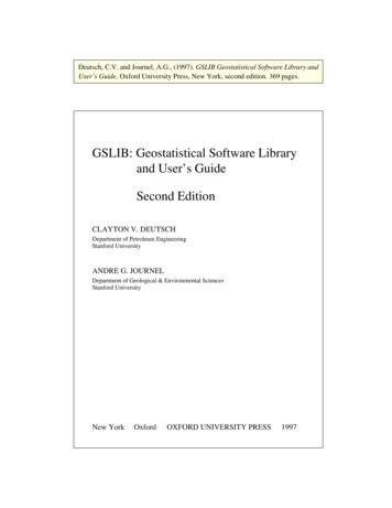
Location Map of Sample DataReference onSimulation
ContentsIIntroductionI.1 About the Source Code . . . . . . . . . . . . . . . . . . . . .II Getting StartedII.1 Geostatistical Concepts: A Review . . . . . . .II.1.1 The Random Function Concept . . . . .II.1.2 Inference and Stationarity . . . . . . . .II.1.3 Variogram . . . . . . . . . . . . . . . . .II.1.4 Kriging . . . . . . . . . . . . . . . . . .II.1.5 Stochastic Simulation . . . . . . . . . .II.2 GSLIB Conventions . . . . . . . . . . . . . . .II.2.1 Computer Requirements . . . . . . . . .II.2.2 Data Files . . . . . . . . . . . . . . . . .II.2.3 Grid Definition . . . . . . . . . . . . . .II.2.4 Program Execution and Parameter FilesII.2.5 Machine Precision . . . . . . . . . . . .II.3 Variogram Model Specification . . . . . . . . .II.3.1 A Straightforward 2D Example . . . . .II.3.2 A 2D Example with Zonal Anisotropy .II.4 Search Strategies . . . . . . . . . . . . . . . . .II.5 Data Sets . . . . . . . . . . . . . . . . . . . . .II.6 Problem Set One: Data Analysis . . . . . . . .III VariogramsIII.1 Measures of Spatial VariabilityIII.2 GSLIB Variogram Programs . .III.3 Regularly Spaced Data gam . .III.4 Irregularly Spaced Data gamv .III.5 Variogram Maps varmap . . . .III.6 Application Notes . . . . . . .III.7 Problem Set Two: 740.4343475053555762
viiiIV KrigingIV.1 Kriging with GSLIB . . . . . . . . . . . . . . .IV.1.1 Simple Kriging . . . . . . . . . . . . . .IV.1.2 Ordinary Kriging . . . . . . . . . . . . .IV.1.3 Kriging with a Trend Model . . . . . . .IV.1.4 Kriging the Trend . . . . . . . . . . . .IV.1.5 Kriging with an External Drift . . . . .IV.1.6 Factorial Kriging . . . . . . . . . . . . .IV.1.7 Cokriging . . . . . . . . . . . . . . . . .IV.1.8 Nonlinear Kriging . . . . . . . . . . . .IV.1.9 Indicator Kriging . . . . . . . . . . . . .IV.1.10Indicator Cokriging . . . . . . . . . . .IV.1.11Probability Kriging . . . . . . . . . . . .IV.1.12Soft Kriging: The Markov-Bayes ModelIV.1.13Block Kriging . . . . . . . . . . . . . . .IV.1.14Cross Validation . . . . . . . . . . . . .IV.2 A Straightforward 2D Kriging Program kb2d .IV.3 A Flexible 3D Kriging Program kt3d . . . . . .IV.4 Cokriging Program cokb3d . . . . . . . . . . .IV.5 Indicator Kriging Program ik3d . . . . . . . .IV.6 Application Notes . . . . . . . . . . . . . . . .IV.7 Problem Set Three: Kriging . . . . . . . . . . .IV.8 Problem Set Four: Cokriging . . . . . . . . . .IV.9 Problem Set Five: Indicator Kriging . . . . . 03106108115116V SimulationV.1 Principles of Stochastic Simulation . . . . . . . .V.1.1 Reproduction of Major Heterogeneities . .V.1.2 Joint Simulation of Several Variables . . .V.1.3 The Sequential Simulation Approach . . .V.1.4 Error Simulation . . . . . . . . . . . . . .V.1.5 Questions of Ergodicity . . . . . . . . . .V.1.6 Going Beyond a Discrete CDF . . . . . .V.2 Gaussian-Related Algorithms . . . . . . . . . . .V.2.1 Normal Score Transform . . . . . . . . . .V.2.2 Checking for Bivariate Normality . . . . .V.2.3 Sequential Gaussian Simulation . . . . . .V.2.4 LU Decomposition Algorithm . . . . . . .V.2.5 The Turning Band Algorithm . . . . . . .V.2.6 Multiple Truncations of a Gaussian FieldV.3 Indicator-Based Algorithms . . . . . . . . . . . .V.3.1 Simulation of Categorical Variables . . . .V.3.2 Simulation of Continuous Variables . . . .V.4 p-Field Simulation . . . . . . . . . . . . . . . . .V.5 Boolean Algorithms . . . . . . . . . . . . . . . 51152155156
CONTENTSixV.6 Simulated Annealing . . . . . . . . . . . . . . . . . . . .V.6.1 Simulation by Simulated Annealing . . . . . . . .V.6.2 Postprocessing with Simulated Annealing . . . .V.6.3 Iterative Simulation Techniques . . . . . . . . . .V.7 Gaussian Simulation Programs . . . . . . . . . . . . . .V.7.1 LU Simulation lusim . . . . . . . . . . . . . . .V.7.2 Sequential Gaussian Simulation sgsim . . . . . .V.7.3 Multiple Truncations of a Gaussian Field gtsim .V.8 Sequential Indicator Simulation Programs . . . . . . . .V.8.1 Indicator Simulation sisim . . . . . . . . . . . .V.8.2 p-Field Simulation pfsim . . . . . . . . . . . . .V.9 A Boolean Simulation Program ellipsim . . . . . . . .V.10 Simulated Annealing Programs . . . . . . . . . . . . . .V.10.1 Simulated Annealing sasim . . . . . . . . . . . .V.10.2 An Annealing Postprocessor anneal . . . . . . .V.11 Application Notes . . . . . . . . . . . . . . . . . . . . .V.12 Problem Set Six: Simulation . . . . . . . . . . . . . . . .VI Other Useful ProgramsVI.1 PostScript Display . . . . . . . . . . . . . . . . . . .VI.1.1 Location Maps locmap . . . . . . . . . . . . .VI.1.2 Gray- and Color-Scale Maps pixelplt . . . .VI.1.3 Histograms and Statistics histplt . . . . . .VI.1.4 Normal Probability Plots probplt . . . . . .VI.1.5 Q-Q and P-P plots qpplt . . . . . . . . . . .VI.1.6 Bivariate Scatterplots and Analysis scatpltVI.1.7 Smoothed Scatterplot Display bivplt . . . .VI.1.8 Variogram Plotting vargplt . . . . . . . . .VI.2 Utility Programs . . . . . . . . . . . . . . . . . . . .VI.2.1 Coordinates addcoord and rotcoord . . . . .VI.2.2 Cell Declustering declus . . . . . . . . . . .VI.2.3 Histogram and Scattergram Smoothing . . .VI.2.4 Random Drawing draw . . . . . . . . . . . .VI.2.5 Normal Score Transformation nscore . . . .VI.2.6 Normal Score Back Transformation backtr .VI.2.7 General Transformation trans . . . . . . . .VI.2.8 Variogram Values from a Model vmodel . . .VI.2.9 Gaussian Indicator Variograms bigaus . . . .VI.2.10Library of Linear System Solvers . . . . . . .VI.2.11Bivariate Calibration bicalib . . . . . . . .VI.2.12Postprocessing of IK Results postik . . . . .VI.2.13Postprocessing of Simulation Results 14222223226227230231232235236239
xCONTENTSA Partial Solutions to Problem SetsA.1 Problem Set One: Data Analysis . .A.2 Problem Set Two: Variograms . . .A.3 Problem Set Three: Kriging . . . . .A.4 Problem Set Four: Cokriging . . . .A.5 Problem Set Five: Indicator KrigingA.6 Problem Set Six: Simulations . . . .241241253266271283296B Software Installation325B.1 Installation . . . . . . . . . . . . . . . . . . . . . . . . . . . . 325B.2 Troubleshooting . . . . . . . . . . . . . . . . . . . . . . . . . . 327C Programming Conventions329C.1 General . . . . . . . . . . . . . . . . . . . . . . . . . . . . . . 329C.2 Dictionary of Variable Names . . . . . . . . . . . . . . . . . . 330C.3 Reference Lists of Parameter Codes . . . . . . . . . . . . . . . 336D Alphabetical Listing of Programs339E List of Acronyms and Notations341E.1 Acronyms . . . . . . . . . . . . . . . . . . . . . . . . . . . . . 341E.2 Common Notation . . . . . . . . . . . . . . . . . . . . . . . . 342Bibliography346Index363
Chapter IIntroductionGSLIB is the name of a directory containing the geostatistical software developed at Stanford. Generations of graduate students have contributed tothis constantly changing collection of programs, ideas, and utilities. Some ofthe most widely used public-domain geostatistical software [58, 62, 72] andmany more in-house programs were initiated from GSLIB. It was decided toopen the GSLIB directory to a wide audience, providing the source code toseed new developments, custom-made application tools, and, it is hoped, newtheoretical advances.What started as a collection of selected GSLIB programs to be distributedon diskette with a minimal user’s guide has turned into a major endeavor;a lot of code has been rewritten for the sake of uniformity, and the user’sguide looks more like a textbook. Yet our intention has been to maintain theoriginal versatility of GSLIB, where clarity of coding prevails over baroquetheory or the search for ultimate speed. GSLIB programs are developmenttools and sketches for custom programs, advanced applications, and research;we expect them to be torn apart and parts grafted into custom softwarepackages.The strengths of GSLIB are also its weaknesses. The flexibility of GSLIB,its modular conception, and its machine independence may assist researchersand those beginners more eager to learn than use; on the other hand, therequirement to make decisions at each step and the lack of a slick user interfacewill frustrate others.Reasonable effort has been made to provide software that is well documented and free of bugs but there is no support or telephone number forusers to call. Each user of these programs assumes the responsibility for theircorrect application and careful testing as appropriate.11 Reports of bugs or significant improvements in the coding should be sent to the authorsat Stanford University.3
4CHAPTER I. INTRODUCTIONTrends in GeostatisticsMost geostatistical theory [63, 118, 188, 195] was established long before theavailability of digital computers allowed its wide application in earth sciences[109, 132, 133]. The development of geostatistics since the late 1960s hasbeen accomplished mostly by application-oriented engineers: They have beenready to bend theory to match the data and their approximations have beenstrengthened by extended theory.Most early applications of geostatistics were related to mapping the spatialdistribution of one or more attributes, with emphasis given to characterizingthe variogram model and using the kriging (error) variance as a measure of estimation accuracy. Kriging, used for mapping, is not significantly better thanother deterministic interpolation techniques that are customized to accountfor anisotropy, data clustering, and other important spatial features of thevariable being mapped [79, 92, 140]. The kriging algorithm also provides anerror variance. Unfortunately, the kriging variance is independent of the datavalues and cannot be used, in general, as a measure of estimation accuracy.Recent applications of geostatistics have de-emphasized the mapping application of kriging. Kriging is now used to build models of uncertainty thatdepend on the data values in addition to the data configuration. The attentionhas shifted from mapping to conditional simulation, also known as stochasticimaging. Conditional simulation allows drawing alternative, equally probablerealizations of the spatial distribution of the attribute(s) under study. Thesealternative stochastic images provide a measure of uncertainty about the unsampled values taken altogether in space rather than one by one. In addition,these simulated images do not suffer from the characteristic smoothing effectof kriging (see frontispiece).Following this trend, the GSLIB software and this guidebook emphasizestochastic simulation tools.Book ContentIncluding this introduction, the book consists of 6 chapters, 5 appendicesincluding a list of programs given, a bibliography, and an index. Two diskettescontaining all the FORTRAN source code are provided.Chapter II provides the novice reader with a review of basic geostatisticalconcepts. The concepts of random functions and stationarity are introducedas models. The basic notations, file conventions, and variogram specificationsused throughout the text and in the software are also presented.Chapter III deals with covariances, variograms, and other more robustmeasures of spatial variability/continuity. The “variogram” programs allowthe simultaneous calculation of many such measures at little added computational cost. An essential tool, in addition to the programs in GSLIB,would be a graphical, highly interactive, variogram modeling program (suchas available in other public-domain software [28, 58, 62]).
5Chapter IV presents the multiple flavors of kriging, from simple and ordinary kriging to factorial and indicator kriging. As already mentioned, krigingcan be used for many purposes in addition to mapping. Kriging can be applied as a filter (Wiener’s filter) to separate either the low-frequency (trend)component or, conversely, the high-frequency (nugget effect) component ofthe spatial variability. When applied to categorical variables or binary transforms of continuous variables, kriging is used to update prior local informationwith neighboring information to obtain a posterior probability distributionfor the unsampled value(s). Notable omissions in GSLIB include kriging withintrinsic random functions of order k (IRF-k) and disjunctive kriging (DK).From a first glance at the list of GSLIB subroutines, the reader may thinkthat other more common algorithms are missing, e.g., kriging with an external drift, probability kriging, and multi-Gaussian kriging. These algorithms,however, are covered by programs named for other algorithms. Kriging withan external drift can be seen as a form of kriging with a trend and is anoption of program kt3d. Probability kriging is a form of cokriging (programcokb3d). As for multi-Gaussian kriging, it is a mere simple kriging (programkt3d) applied to normal score transforms of the data (program nscore) followed by an appropriate back transform of the estimates.Chapter V presents the principles and various algorithms for stochasticsimulation. Major heterogeneities, possibly modeled by categorical variables,should be simulated first; then continuous properties are simulated withineach reasonably homogeneous category. It is recalled that fluctuations of therealization statistics (histogram, variograms, etc.) are expected, particularlyif the field being simulated is not very large with respect to the range(s)of correlation. Stochastic simulation is currently the most vibrant field ofresearch in geostatistics, and the list of algorithms presented in this text andcoded in GSLIB is not exhaustive. GSLIB includes only the most commonlyused stochastic algorithms as of 1996. Physical process simulations [179], thevast variety of object-based algorithms [174], and spectral domain algorithms[18, 28, 76, 80] are not covered here, notwithstanding their theoretical andpractical importance.Chapter VI proposes a number of useful utility programs including some togenerate graphics in the PostScript page description language. Seasoned userswill already have their own programs. Similar utility programs are availablein classical textbooks or in inexpensive statistical software. These programshave been included, however, because they are essential to the practice ofgeostatistics. Without a histogram and scatterplot, summary statistics, andother displays there would be no practical geostatistics; without a declustering program most geostatistical studies would be flawed from the beginning;without normal score transform and back transform programs there would beno multi-Gaussian geostatistics; an efficient and robust linear system solveris essential to any kriging exercise.Each chapter starts with a brief summary and a first section on methodology (II.1, III.1, IV.1, and V.1). The expert geostatistician may skip this first
6CHAPTER I. INTRODUCTIONsection, although it is sometimes useful to know the philosophy underlying thesoftware being used. The remaining sections in each chapter give commentedlists of input parameters for each subroutine. A section entitled “ApplicationNotes” is included near the end of each chapter with useful advice on usingand improving the programs.Chapters II through V end with sections suggesting one or more problemsets. These problems are designed to provide a first acquaintance with themost important GSLIB programs and a familiarity with the parameter filesand notations used. All problem sets are based on a common synthetic dataset provided with the GSLIB distribution diskettes. The questions asked areall open-ended; readers are advised to pursue their investigations beyond thequestions asked. Limited solutions to each problem set are given in AppendixA; they are not meant to be definitive general solutions. The first time aprogram is encountered the input parameter file is listed along with the firstand last 10 lines of the corresponding output file. These limited solutionsare intended to allow readers to check their understanding of the programinput and output. Working through the problem sets before referring tothe solutions will provide insight into the algorithms. Attempting to applyGSLIB programs (or any geostatistical software) directly to a real-life problemwithout some prior experience may be extremely frustrating.I.1About the Source CodeThe source code provided in GSLIB adheres as closely as possibly to theANSI standard FORTRAN 77 programming language. FORTRAN was retained chiefly because of its familiarity and common usage. Some considerFORTRAN the dinosaur of programming languages when compared withnewer object-oriented programming languages; nevertheless, FORTRAN remains a viable and even desirable scientific programming language due to itssimplicity and the introduction of better features in new ANSI standards oras enhancements by various software companies.GSLIB was coded to the ANSI standard to achieve machine independence.We did not want the use of GSLIB limited to any specific PC, workstation,or mainframe computer. Many geostatistical exercises may be performed ona laptop PC. Large stochastic simulations and complex modeling, however,would be better performed on a more powerful machine. GSLIB programshave been compiled on machines ranging from an XT clone to the latest multiple processor POWER Challenge. No executable programs are provided;only ASCII files containing the source code and other necessary input filesare included in the enclosed diskettes. The source code can immediately bedismantled and incorporated into custom programs, or compiled and usedwithout modification. Appendix B contains detailed information about software installation and troubleshooting.The 1978 ANSI FORTRAN 77 standard does not allow dynamic memoryallocation. This poses an inconvenience since array dimensioning and memory
I.1. ABOUT THE SOURCE CODE7allocation must be hardcoded in all programs. To mitigate this inconvenience,the dimensioning and memory allocation have been specified in an “include”file. The include file is common to all necessary subroutines. Therefore,the array dimensioning limits, such as the maximum number of data or themaximum grid size, has to be changed in only one file.Although the maximum dimensioning parameters are hardcoded in an include file, it is clearly undesirable to use this method to specify most inputparameters. Given the goal of machine independence, it is also undesirableto have input parameters enter the program via a menu-driven graphical userinterface. For these reasons the input parameters are specified in a prepared“parameter” file. These parameter files must follow a specified format. Anadvantage of this form of input is that the parameter files provide a permanent record of run parameters. With a little experience users will find thepreparation and modification of parameter files faster than most other formsof parameter input. Machine-dependent graphical user interfaces would bean alternative.Further, the source code for any specific program has been separated intoa main program and then all the necessary subroutines. This was done tofacilitate the isolation of key subroutines for their incorporation into customsoftware packages. In general, there are four computer files associated withany algorithm or program: the main program, the subroutines, an includefile, and a parameter file.Most program operations are separated into short, easily understood, program modules. Many of these shorter subroutines and funtions are then usedin more than one program. Care has been taken to use a consistent formatwith a statement of purpose, a list of the input parameters, and a list ofprogrammers who worked on a given piece of code. Extensive in-line comments explain the function of the code and identify possible enhancements.A detailed description of the programming conventions and a dictionary ofthe variable names are given in Appendix C.
8CHAPTER I. INTRODUCTION
Chapter IIGetting StartedThis chapter provides a brief review of the geostatistical concepts underlyingGSLIB and an initial presentation of notations, conventions, and computerrequirements.Section II.1 establishes the derivation of posterior probability distributionmodels for unsampled values as a principal goal. From such distributions, bestestimates can be derived together with probability intervals for the unknowns.Stochastic simulation is the process of Monte Carlo drawing of realizationsfrom such posterior distributions.Section II.2 gives some of the basic notations, computer requirements, andfile conventions used throughout the GSLIB text and software.Section II.3 considers the important topic of variogram modeling. Thenotation and conventions established in this section are consistent throughoutall GSLIB programs.Section II.4 considers the different search strategies that are implementedin GSLIB. The super block search, spiral search, two-part search, and the useof covariance lookup tables are discussed.Section II.5 introduces the data set that will be used throughout fordemonstration purposes. A first problem set is provided in Section II.6 toacquaint the reader with the data set and the utility programs for exploratorydata analysis.II.1Geostatistical Concepts: A ReviewGeostatistics is concerned with “the study of phenomena that fluctuate inspace ” and/or time ([146], p. 31). Geostatistics offers a collection of deterministic and statistical tools aimed at understanding and modeling spatialvariability.The basic paradigm of predictive statistics is to characterize any unsampled (unknown) value z as a random variable (RV) Z, the probability distribution of which models the uncertainty about z. A random variable is a9
10CHAPTER II. GETTING STARTEDvariable that can take a variety of outcome values according to some probability (frequency) distribution. The random variable is traditionally denotedby a capital letter, say Z, while its outcome values are denoted with thecorresponding lower-case letter, say z or z (l) . The RV model Z, and morespecifically its probability distribution, is usually location-dependent; hencethe notation Z(u), with u being the location coordinates vector. The RVZ(u) is also information-dependent in the sense that its probability distribution changes as more data about the unsampled value z(u) become available.Examples of continuously varying quantities that can be effectively modeledby RVs include petrophysical properties (porosity, permeability, metal or pollutant concentrations) and geographical properties (topographic elevations,population densities). Examples of categorical variables include geologicalproperties such as rock types or counts of insects or fossil species.The cumulative distribution function (cdf) of a continuous RV Z(u) isdenoted:F (u; z) Prob {Z(u) z}(II.1)When the cdf is made specific to a particular information set, for example(n) consisting of n neighboring data values Z(uα ) z(uα ), α 1, . . . , n,the notation “conditional to (n)” is used, defining the conditional cumulativedistribution function (ccdf):F (u; z (n)) Prob {Z(u) z (n)}(II.2)In the case of a categorical RV Z(u) that can take any one of K outcomevalues k 1, . . . , K, a similar notation is used:F (u; k (n)) Prob {Z(u) k (n)}(II.3)Expression (II.1) models the uncertainty about the unsampled value z(u)prior to using the information set (n); expression (II.2) models the posterioruncertainty once the information set (n) has been accounted for. The goal,implicit or explicit, of any predictive algorithm is to update prior models ofuncertainty such as (II.1) into posterior models such as (II.2). Note that theccdf F (u; z (n)) is a function of the location u, the sample size and geometricconfiguration (the data locations uα , α 1, . . . , n), and the sample values[the n values z(uα )s].From the ccdf (II.2) one can derive different optimal estimates for theunsampled value z(u) in addition to the ccdf mean, which is the least-squareserror estimate. One can also derive various probability intervals such as the95% interval [q(0.025);q(0.975)] such thatProb {Z(u) [q(0.025); q(0.975)] (n)} 0.95with q(0.025) and q(0.975) being the 0.025 and 0.975 quantiles of the ccdf,for example,q(0.025) is such that F (u; q(0.025) (n)) 0.025
II.1. GEOSTATISTICAL CONCEPTS: A REVIEW11Moreover, one can draw any number of simulated outcome values z (l) (u), l 1, . . . , L, from the ccdf
GSLIB is the name of a directory containing the geostatistical software de-veloped at Stanford. Generations of graduate students have contributed to this constantly changing collection of programs, ideas, and utilities. Some of the most widely used public-domain geostatistical software [58, 62, 72] and