Transcription
ArcGIS 9 Using ArcGIS Geostatistical Analyst
Copyright 2001, 2003 ESRIAll Rights Reserved.Printed in the United States of America.The information contained in this document is the exclusive property of ESRI. This work is protected under United States copyright law and the copyrightlaws of the given countries of origin and applicable international laws, treaties, and/or conventions. No part of this work may be reproduced or transmittedin any form or by any means, electronic or mechanical, including photocopying or recording, or by any information storage or retrieval system, except asexpressly permitted in writing by ESRI. All requests should be sent to Attention: Contracts Manager, ESRI, 380 New York Street, Redlands, CA 923738100, USA.The information contained in this document is subject to change without notice.DATA CREDITSCarpathian Mountains data supplied by USDA Forest Service, Riverside, California, and is used here with permission.Radioceasium data supplied by International Sakharov Environmental University, Minsk, Belarus, and is used here with permission. Copyright 1996.Air quality data for California supplied by California Environmental Protection Agency, Air Resource Board, and is used here with permission.Copyright 1997.Radioceasium contamination in forest berries data supplied by the Institute of Radiation Safety “BELRAD”, Minsk, Belarus, and is used here withpermission. Copyright 1996.CONTRIBUTING WRITERSKevin Johnston, Jay M. Ver Hoef, Konstantin Krivoruchko, and Neil LucasDATA DISCLAIMERTHE DATA VENDOR(S) INCLUDED IN THIS WORK IS AN INDEPENDENT COMPANY AND, AS SUCH, ESRI MAKES NO GUARANTEES AS TO THEQUALITY, COMPLETENESS, AND/OR ACCURACY OF THE DATA. EVERY EFFORT HAS BEEN MADE TO ENSURE THE ACCURACY OF THE DATAINCLUDED IN THIS WORK, BUT THE INFORMATION IS DYNAMIC IN NATURE AND IS SUBJECT TO CHANGE WITHOUT NOTICE. ESRI ANDTHE DATA VENDOR(S) ARE NOT INVITING RELIANCE ON THE DATA, AND ONE SHOULD ALWAYS VERIFY ACTUAL DATA AND INFORMATION.ESRI DISCLAIMS ALL OTHER WARRANTIES OR REPRESENTATIONS, EITHER EXPRESSED OR IMPLIED, INCLUDING, BUT NOT LIMITED TO,THE IMPLIED WARRANTIES OF MERCHANTABILITY OR FITNESS FOR A PARTICULAR PURPOSE. ESRI AND THE DATA VENDOR(S) SHALLASSUME NO LIABILITY FOR INDIRECT, SPECIAL, EXEMPLARY, OR CONSEQUENTIAL DAMAGES, EVEN IF ADVISED OF THE POSSIBILITYTHEREOF.U. S. GOVERNMENT RESTRICTED/LIMITED RIGHTSAny software, documentation, and/or data delivered hereunder is subject to the terms of the License Agreement. In no event shall the U.S. Government acquiregreater than RESTRICTED/LIMITED RIGHTS. At a minimum, use, duplication, or disclosure by the U.S. Government is subject to restrictions as set forth inFAR §52.227-14 Alternates I, II, and III (JUN 1987); FAR §52.227-19 (JUN 1987) and/or FAR §12.211/12.212 (Commercial Technical Data/ComputerSoftware); and DFARS §252.227-7015 (NOV 1995) (Technical Data) and/or DFARS §227.7202 (Computer Software), as applicable. Contractor/Manufactureris ESRI, 380 New York Street, Redlands, CA 92373-8100, USA.ESRI, SDE, the ESRI globe logo, ArcGIS, ArcInfo, ArcCatalog, ArcMap, 3D Analyst, and GIS by ESRI are trademarks, registered trademarks, or service marksof ESRI in the United States, the European Community, and certain other jurisdictions.Other companies and products mentioned herein are trademarks or registered trademarks of their respective trademark owners.Attribution.pmd111/25/2003, 4:46 PM
Contents1 Welcome to ArcGIS Geostatistical Analyst1Exploratory spatial data analysis 2Semivariogram modeling 3Surface prediction and error modeling 4Threshold mapping 5Model validation and diagnostics 6Surface prediction using cokriging 7Tips on learning Geostatistical Analyst 82 Quick-start tutorial11Introduction to the tutorial 12Exercise 1: Creating a surface using default parameters 14Exercise 2: Exploring your data 19Exercise 3: Mapping ozone concentration 26Exercise 4: Comparing models 38Exercise 5: Mapping the probability of ozone exceeding a critical thresholdExercise 6: Producing the final map 423 The principles of geostatistical analysis3949Understanding deterministic methods 50Understanding geostatistical methods 53Working through a problem 54Basic principles behind geostatistical methods 59Modeling a semivariogram 61Kriging 74A guide to the Geostatistical Analyst extension 784Exploratory Spatial Data Analysis81What is Exploratory Spatial Data Analysis? 82Exploratory Spatial Data Analysis 83Exploratory Spatial Data Analysis tools 84Examining the distribution of the data 95iiiTOC.p65303/07/2001, 4:00 PM
Examining the distribution of your data 98Looking for global and local outliers 99Identifying global and local outliers 101Looking for global trends 103Looking for global trends 105Examining spatial autocorrelation and directional variation 106Examining spatial structure and directional variation 108Understanding covariation among multiple datasets 109Understanding spatial covariation among multiple datasets 1115 Deterministic methods for spatial interpolation12113How Inverse Distance Weighted interpolation works 114Creating a map using IDW 118How global polynomial interpolation works 120Creating a map using global polynomial interpolation 122How local polynomial interpolation works 123Creating a map using local polynomial interpolation 125How radial basis functions work 126Creating a map using RBFs 1296 Creating a surface with geostatistical techniques131What are geostatistical interpolation techniques? 132Understanding the different kriging models 133Understanding output surface types 135Creating a kriging map using defaults 136Understanding transformations and trends 137Understanding ordinary kriging 138Creating a map using ordinary kriging 139Understanding simple kriging 143Creating a map using simple kriging 144Understanding universal kriging 150ivTOC.p65USING ARCGIS GEOSTATISTICAL ANALYST403/07/2001, 4:00 PM
Creating a map using universal kriging 151Understanding thresholds 153Understanding indicator kriging 154Creating a map using indicator kriging 155Understanding probability kriging 156Creating a map using probability kriging 157Understanding disjunctive kriging 159Creating a map using disjunctive kriging 160Understanding cokriging 165Creating a map using cokriging 1667Using analytical tools when generating surfaces167Investigating spatial structure: variography 168Modeling semivariograms and covariance functions 175Determining the neighborhood search size 181Determining the neighborhood search size 185Performing cross-validation and validation 189Performing cross-validation to assess parameter selections 193Assessing decision protocol using validation 195Comparing one model with another 197Comparing one model with another 199Modeling distributions and determining transformations 200Using transformations (log, Box Cox, and arcsine) 204Using the normal score transformation 205Checking for the bivariate normal distribution 206Checking for bivariate distribution 209Implementing declustering to adjust for preferential sampling 211Declustering to adjust for preferential sampling 214Removing trends from the data 216Removing global and local trends from the data: detrending 218CONTENTSTOC.p65v503/07/2001, 4:00 PM
8Displaying and managing geostatistical layersWhat is a geostatistical layer? 220Adding layers 222Working with layers in a map 223Managing layers 224Viewing geostatistical layers in ArcCatalog 225Representing a geostatistical layer 227Changing the symbology of a geostatistical layer 229Data classification 230Classifying data 233Setting the scales at which a geostatistical layer will be displayedPredicting values for locations outside the area of interest 236Saving and exporting geostatistical layers 2379 Additional geostatistical analysis tools219235239Changing the parameters of a geostatistical layer: method properties 240Predicting values for specified locations 241Performing validation on a geostatistical layer created from a subset 243Appendix A247Appendix B275Glossary279ReferencesIndex285287viTOC.p65USING ARCGIS GEOSTATISTICAL ANALYST603/07/2001, 4:00 PM
Welcome to ArcGIS Geostatistical AnalystIN THIS CHAPTER Exploratory spatial data analysis Semivariogram modeling Surface prediction and errormodeling Threshold mapping Model validation and diagnostics Surface prediction using cokriging Tips on learning GeostatisticalAnalyst1Welcome to the ESRI ArcGIS Geostatistical Analyst extension foradvanced surface modeling using deterministic and geostatistical methods.Geostatistical Analyst extends ArcMap by adding an advanced toolbarcontaining tools for exploratory spatial data analysis and a geostatisticalwizard to lead you through the process of creating a statistically validsurface. New surfaces generated with Geostatistical Analyst cansubsequently be used in geographic information system (GIS) models and invisualization using ArcGIS extensions such as ArcGIS Spatial Analyst andArcGIS 3D Analyst .Geostatistical Analyst is revolutionary because it bridges the gap betweengeostatistics and GIS. For some time, geostatistical tools have beenavailable, but never integrated tightly within GIS modeling environments.Integration is important because, for the first time, GIS professionals canbegin to quantify the quality of their surface models by measuring thestatistical error of predicted surfaces.Surface fitting using Geostatistical Analyst involves three key steps(demonstrated on the following pages): Exploratory spatial data analysis Structural analysis (calculation and modeling of the surface properties ofnearby locations) Surface prediction and assessment of resultsThe software contains a series of easy-to-use tools and wizards that guideyou through each of these steps. It also includes a number of unique toolsfor statistical spatial data analysis.1ch01 Welcome.pmd111/25/2003, 2:54 PM
Exploratory spatial data analysisUsing measured sample points from a study area, Geostatistical Analyst can create accurate predictions for other unmeasured locationswithin the same area. Exploratory spatial data analysis tools included with Geostatistical Analyst are used to assess the statisticalproperties of data such as spatial data variability, spatial data dependence, and global trends.A number of exploratory spatial data analysis tools are used to investigate the properties of ozone measurements takenat monitoring stations in the Carpathian Mountains.2Welcome.p65USING ARCGIS GEOSTATISTICAL ANALYST203/05/2001, 2:27 PM
Semivariogram modelingGeostatistical analysis of data occurs in two phases: 1) modeling the semivariogram or covariance to analyze surface properties, and2) kriging. A number of kriging methods are available for surface creation in Geostatistical Analyst, including ordinary, simple,universal, indicator, probability, and disjunctive kriging.The two phases of geostatistical analysis of data are illustrated above. First, the semivariogram/covariance wizard was used tofit a model to winter temperature data for the USA. This model was then used to create the temperature distribution map.WELCOME TO ARCGIS GEOSTATISTICAL ANALYSTWelcome.p653303/05/2001, 2:27 PM
Surface prediction and error modelingVarious types of map layers can be produced using Geostatistical Analyst, including prediction maps, quantile maps, probability maps,and prediction standard error maps.Here, Geostatistical Analyst has been used to produce a prediction map of radioceasium soil contamination levels in the country ofBelarus after the Chernobyl nuclear power plant accident.4Welcome.p65USING ARCGIS GEOSTATISTICAL ANALYST43/21/01, 7:58 AM
Threshold mappingProbability maps can be generated to predict where values exceed a critical threshold.Locations shown in dark orange and red indicate a probability greater than 62.5% that radioceasium contamination exceeds the upperpermissible level (critical threshold) in forest berries.WELCOME TO ARCGIS GEOSTATISTICAL ANALYSTWelcome.p655503/05/2001, 2:27 PM
Model validation and diagnosticsInput data can be split into two subsets. The first subset of the available data can be used to develop a model for prediction. Thepredicted values are then compared with the known values at the remaining locations using the Validation tool.The validation wizard is used to assess a model developed to predict organic matter for a farm in Illinois.6Welcome.p65USING ARCGIS GEOSTATISTICAL ANALYST603/05/2001, 2:27 PM
Surface prediction using cokrigingCokriging, an advanced surface modeling method included in Geostatistical Analyst, can be used to improve surface prediction of aprimary variable by taking into account secondary variables, provided that the primary and secondary variables are spatially correlated.In this example, exploratory spatial data analysis tools are used to explore spatial correlation betweenozone (primary variable) and nitrogen dioxide (secondary variable) in California. Because the variables arespatially correlated, cokriging can use the nitrogen dioxide data to improve predictions when mappingozone.Additionally, Geostatistical Analyst contains a number of unique tools to improve prediction, including tools for data transformation;data detrending using local polynomial interpolation; identification of the shift parameter in a cross-covariance model; error modelingto define the proportion of error resulting from microscale variations and measurement errors; examination of data for bivariatedistribution; optimal searching neighborhood selection; and quantile map production.WELCOME TO ARCGIS GEOSTATISTICAL ANALYSTWelcome.p65773/21/01, 8:01 AM
Tips on learning GeostatisticalAnalystIf you are new to the concept of geostatistics, remember that youdon t have to know everything about Geostatistical Analyst to getimmediate results. Begin learning Geostatistical Analyst byreading Chapter 2, Quick-start tutorial . This chapter introducesyou to some of the tasks you can accomplish using GeostatisticalAnalyst and provides an excellent starting point as you begin tothink about how to tackle your own spatial problems.Geostatistical Analyst comes with the data used in the tutorial, soyou can follow along step by step at your computer.If you prefer to jump right in and experiment on your own, useChapter 5, Deterministic methods for spatial interpolation , andChapter 6, Creating a surface with geostatistical techniques , asa guide to learn the concepts and the steps to perform a certaintask.Finding answers to questionsLike most people, your goal is to complete your tasks whileinvesting a minimum amount of time and effort on learning howto use software. You want intuitive, easy-to-use software thatgives you immediate results without having to read pages ofdocumentation. However, when you do have a question, you wantthe answer quickly so you can complete your task. That s whatthis book is all about getting the answers you need, when youneed them.This book describes geostatistical analysis tasks from basic toadvanced that you ll perform with Geostatistical Analyst.Although you can read this book from start to finish, you ll likelyuse it more as a reference. When you want to know how to do aparticular task, such as identifying global outliers, just look it upin the table of contents or the index. What you ll find is aconcise, step-by-step description of how to complete the task.Some chapters also include detailed information that you can8Welcome.p65read if you want to learn more about the concepts behind thetasks. You may also refer to the glossary in this book if you comeacross any unfamiliar geostatistical terms or need to refresh yourmemory.About this bookThis book is designed to help you perform geostatistical analysesby giving you conceptual information and teaching you how toperform tasks to solve your geostatistical problems. Topicscovered in Chapter 2 assume you are familiar with thefundamentals of a Geographic Information System (GIS) andhave a basic knowledge of ArcGIS. If you are new to GIS orArcMap, you are encouraged to take some time to read GettingStarted with ArcGIS and Using ArcMap, which you received inyour ArcGIS package. It is not necessary to do so to continuewith this book; simply use the books as references.Chapter 3 takes you through the basic principles of geostatistics,helping you understand the different interpolation methods andhow they work conceptually. Chapter 4 covers the variousESDAs that allow you to understand your data better. Chapter 5explains the deterministic interpolation methods. Chapter 6discusses the various geostatistical methods, and Chapter 7discusses the wide variety of tools that you use when performinginterpolation. Chapter 8 describes the various display andmanagement tools that are applicable to geostatistical layers.Chapter 9 covers a series of other geostatistical analysisconcepts and tasks. Appendix A provides detailed mathematicalformulas for the various functions and methods used inGeostatistical Analyst. Finally, a glossary gives definitions tovarious geostatistical terms used in this book.Getting help on your computerIn addition to this book, use the ArcMap online Help system tolearn how to use Geostatistical Analyst and ArcMap. To learnhow to use Help, see the book Using ArcMap.USING ARCGIS GEOSTATISTICAL ANALYST803/05/2001, 2:27 PM
Contacting ESRIIf you need to contact ESRI for technical support, see the productregistration and support card you received with ArcGISGeostatistical Analyst, or refer to Contacting Technical Support in the Getting more help section of the ArcGIS Desktop Helpsystem. You can also visit ESRI on the Web at www.esri.com andsupport.esri.com for more information on Geostatistical Analystand ArcGIS.ESRI education solutionsESRI provides educational opportunities related to geographicinformation science, GIS applications, and technology. You canchoose among instructor-led courses, Web-based courses, andself-study workbooks to find education solutions that fit yourlearning style. For more information, go to www.esri.com/education.WELCOME TO ARCGIS GEOSTATISTICAL ANALYSTch01 Welcome.p659908/28/2002, 1:25 PM
Welcome.p651003/05/2001, 2:27 PM
2Quick-start tutorialIN THIS CHAPTER Exercise 1: Creating a surfaceusing default parameters Exercise 2: Exploring your data Exercise 3: Mapping ozone concentrationWith Geostatistical Analyst, you can easily create a continuous surface,or map, from measured sample points stored in a point-feature layer, rasterlayer, or by using polygon centroids. The sample points may be measurementssuch as elevation, depth to the water table, or levels of pollution, as is the casein this tutorial. When used in conjunction with ArcMap, Geostatistical Analystprovides a comprehensive set of tools for creating surfaces that can be usedto visualize, analyze, and understand spatial phenomena.Tutorial scenario Exercise 4: Comparing models Exercise 5: Mapping the probability of ozone exceeding a criticalthreshold Exercise 6: Producing the finalmapThe U.S. Environmental Protection Agency is responsible for monitoringatmospheric ozone concentration in California. Ozone concentration is measured at monitoring stations throughout the state.The locations of the stations are shown here. Theconcentration levels of ozone are known forall of the stations, but we are also interested inknowing the level for every location in California.However, due to cost and practicality, monitoringstations cannot be everywhere. GeostatisticalAnalyst provides tools that make the best predictions possible by examining the relationshipsbetween all of the sample points and producing acontinuous surface of ozone concentration,standard errors (uncertainty) of predictions, andprobabilities that critical values are exceeded.11ch02 Tutorial.pmd1111/25/2003, 4:33 PM
Introduction to the tutorialThe data you ll need for this tutorial is included on theGeostatistical Analyst installation disk. The datasets wereprovided courtesy of the California Air Resources Board.using the ESDA tools and working with the geostatisticalparameters, you will be able to create a more accuratesurface.The datasets are:Many times it is not the actual values of some caustichealth risk that is of concern, but rather if it is above sometoxic level. If this is the case immediate action must betaken. The third surface you create will assess the probability that a critical ozone threshold value has been exceeded.DatasetDescriptionca outlineOutline map of Californiaca ozone ptsOzone point samples (ppm)ca citiesLocation of major Californian citiesca hillshadeA hillshade map of CaliforniaThe Ozone dataset (ca ozone pts) represents the 1996maximum eight-hour average concentration of ozone inparts per million (ppm). (The measurements were takendaily and grouped into eight-hour blocks.) The original datahas been modified for the purposes of the tutorial andshould not be taken to be accurate data.From the ozone point samples (measurements), you willproduce two continuous surfaces (maps), predicting thevalues of ozone concentration for every location in the Stateof California based on the sample points that you have. Thefirst map that you create will simply use all default optionsto show you how easy it is to create a surface from yoursample points. The second map that you produce will allowyou to incorporate more of the spatial relationships that arediscovered among the points. When creating this secondmap, you will use the ESDA tools to examine your data.You will also be introduced to some of the geostatisticaloptions that you can use to create a surface such asremoving trends and modeling spatial autocorrelation. ByFor this tutorial, the critical threshold will be if the maximumaverage of ozone goes above 0.12 ppm in any eight-hourperiod during the year; then the location should be closelymonitored. You will use the Geostatistical Analyst to predictthe probability of values complying with this standard.This tutorial is divided into individual tasks that are designedto let you explore the capabilities of the GeostatisticalAnalyst at your own pace. To get additional help, explorethe ArcMap online Help system or see Using ArcMap.12Tutorial.p65USING ARCGIS GEOSTATISTICAL ANALYST1203/07/2001, 2:38 PM
Exercise 1 takes you through accessing the Geostatistical Analyst and through the process of creating asurface of ozone concentration to show you how easy itis to create a surface using the default parameters. Exercise 2 guides you through the process of exploringyour data before you create the surface in order to spotoutliers in the data and to recognize trends. Exercise 3 creates the second surface that considersmore of the spatial relationships discovered in Exercise 2and improves on the surface you created in Exercise 1.This exercise also introduces you to some of the basicconcepts of geostatistics. Exercise 4 shows you how to compare the results of thetwo surfaces that you created in Exercises 1 and 3 inorder to decide which provides the better predictions ofthe unknown values. Exercise 5 takes you through the process of mapping theprobability that ozone exceeds a critical threshold, thuscreating the third surface. Exercise 6 shows you how to present the surfaces youcreated in Exercises 3 and 5 for final display, usingArcMap functionality.You will need a few hours of focused time to complete thetutorial. However, you can also perform the exercises oneat a time if you wish, saving your results after each exercise.QUICK-START TUTORIALTutorial.p65131303/07/2001, 2:38 PM
Exercise 1: Creating a surface using default parametersBefore you begin you must first start ArcMap and enableGeostatistical Analyst.Starting ArcMap and enable Geostatistical AnalystClick the Start button on the Windows taskbar, point toPrograms, point to ArcGIS, and click ArcMap. In ArcMap,click Tools, click Extensions, and check GeostatisticalAnalyst. Click Close.1574Adding the Geostatistical Analyst toolbar toArcMapClick View, point to Toolbars, and click GeostatisticalAnalyst.Adding data layers to ArcMapOnce the data has been added, you can use ArcMap todisplay the data and, if necessary, to change the propertiesof each layer (symbology, and so on).1. Click the Add Data button on the Standard toolbar.2. Navigate to the folder where you installed the tutorialdata (the default installation path isC:\ArcGIS\ArcTutor\Geostatistics), hold down the Ctrlkey, then click and highlight the ca ozone pts andca outline datasets.3. Click Add.4. Click the ca outline layer legend in the table of contentsto open the Symbol Selector dialog box.5. Click the Fill Color dropdown arrow and click No Color.6. Click OK on the Symbol Selector dialog box.6The ca outline layer is now displayed transparently withjust the outline visible. This allows you to see the layersthat you will create in this tutorial underneath this layer.Saving your mapIt is recommended that you save your map after eachexercise.7. Click the Save button on the Standard toolbar.You will need to provide a name for the map becausethis is the first time you have saved it (we suggestOzone Prediction Map.mxd). To save in the future, clickSave.14Tutorial.p65USING ARCGIS GEOSTATISTICAL ANALYST1403/07/2001, 2:38 PM
Creating a surface using the defaults23Next you will create (interpolate) a surface of ozoneconcentration using the default settings of the GeostatisticalAnalyst. You will use the ozone point dataset(ca ozone pts) as the input dataset and interpolate theozone values at the locations where values are not knownusing ordinary kriging. You will click Next in many of thedialog boxes, thus accepting the defaults. Do not worryabout the details of the dialog boxes in this exercise. Eachdialog box will be revisited in later exercises. The intent ofthis exercise is to create a surface using the default options.1. Click the Geostatistical Analyst toolbar, then clickGeostatistical Wizard.1456. Click Next on the Geostatistical Method Selection dialogbox.2. Click the Input Data dropdown arrow and clickca ozone pts.3. Click the Attribute dropdown arrow and click theOZONE attribute.4. Click Kriging in the Methods dialog box.5. Click Next.By default, Ordinary Kriging and Prediction Map will beselected in the Geostatistical Method Selection dialogbox.Note that having selected the method to map the ozonesurface, you could click Finish here to create a surfaceusing the default parameters. However, steps 6 to 10 willexpose you to many of the different dialog boxes.6QUICK-START TUTORIALTutorial.p65151503/07/2001, 2:38 PM
7The Semivariogram/Covariance Modeling dialog box allowsyou to examine spatial relationships between measuredpoints. You assume things that are close are more alike.The semivariogram allows you to explore this assumption.The process of fitting a semivariogram model while capturing the spatial relationships is known as variography.7. Click Next.8The crosshairs show a location that has no measured value.To predict a value at the crosshairs you can use the valuesat the measured locations. You know that the values of thecloser measured locations are more like the value of theunmeasured location that you are trying to predict. The redpoints in the above image are going to be weighted (orinfluence the unknown value) more than the green pointssince they are closer to the location you are predicting.Using the surrounding points, with the model fitted in theSemivariogram Modeling dialog box, you can predict amore accurate value for the unmeasured location.8. Click Next.16Tutorial.p65USING ARCGIS GEOSTATISTICAL ANALYST163/21/01, 8:02 AM
Q9WThe Cross Validation dialog box gives you some idea of how well the model predicts the values at the unknownlocations. You will learn how to use the graph and understand the statistics in Exercise 4.9. Click Finish.The Output Layer Information dialog box summarizesinformation on the method (and its associated parameters) that will be used to create the output surface.10. Click OK.The predicted ozone map will appear as the top layer inthe table of contents.11. Click the layer in the table of contents to highlight it,then click again, and change the layer name to Default .This name change will help you distinguish this layerfrom the one you will create in Exercise 4.12. Click save on the ArcMap Standard toolbar.Notice that the interpolation continues into the ocean. Youwill learn in Exercise 6 how to restrict the predictionsurface to stay within California.QUICK-START TUTORIALTutorial.p6517173/21/01, 8:02 AM
Surface-fitting methodologyYou have now created a map of ozone concentration and completed Exercise 1 of the tutorial. While it is a simple task tocreate a map (surface) using the Geostatistical Analyst, it is important to follow a structured process as shown below:Exercise 1Representthe dataAdd layers and display them in the ArcMap data view.Exercise 2Explorethe dataInvestigate the statistical properties of your dataset. These tools can be usedto investigate the data, whether or not the intention is to create a surface.Exercise 3Fit amodelSelect a model to create a surface. The exploratory data phase will help inthe selection of an appropriate model.Exercise 3PerformdiagnosticsAssess the output surface. This will help you understand how well the model predicts the unknown values.Exercise 4Comparethe modelsIf more than one surface is produced, the results can becompared and a decision made as to which provides the betterpredictions of unknown values.You will follow this structured process in the following exercises of the tutorial. In addition, in Exercise 5, you will create asurface of those locations that exceed a specified threshold and, in Exercise 6, you will create a final presentation layout ofthe results of the analysis performed in the tutorial.Note that you have already performed the first step of this process, representing the data, in Exercise 1. In E
in this tutorial. When used in conjunction with ArcMap, Geostatistical Analyst provides a comprehensive set of tools for creating surfaces that can be used to visualize, analyze, and understand spatial phenomena. Tutorial scenario The U.S. Environmental Protection Agency is responsible for monitoring atmospheric ozone concentration in California.