Transcription
Integration of Geostatistical Modeling with History Matching:Global and Regional PerturbationOliveira, Gonçalo SoaresSoares, Amílcar Oliveira (CERENA/IST)Schiozer, Denis José (UNISIM/UNICAMP)IntroductionOne of the most important activities developed by reservoir engineers is the ability to makeprevisions about the expected behave of the reservoir in the life time of the field. This prevision is doneafter the calibration of history data taking into account all data available in the field (seismic, well logs,cores, etc). Even though the engineer can model a reservoir that fully respects all information andproduction data, a set of models must be done because although they can reproduce the same historydata, they will probably make different previsions. Once the models are created, a quantification ofuncertainty and risk can be done, helping management and decision making.History matching is an important process in the management of a petroleum reservoir. Theglobal framework to work with history matching is done by minimizing the value of an objective functionwhich quantifies the mismatch between the history data and the data simulated.To minimize the value of the objective function, an iterative process is done by changingdifferent parameters of the reservoir in order to obtain a better answer from the model. Theseparameters can include static properties like porosity, permeability or net-gross, or even parametersfrom the flow simulator, like oil-water contact, rock compressibility and relative permeability.In the last few years, the importance of integrating geostatistical modeling with historymatching has increased. Geostatistics has the advantage of allowing the user to create multiple imagesof the reservoir, making possible to quantify uncertainty, while honoring all the well data.The main objective of this work is to develop a method that can be included in the loop of theiterative process of the history matching, by shorting the range of different answers that heterogeneitygives in the simulation. A main preoccupation of the work is the possibility for it to be used in industryand reproduced easily, using only software available in companies.Is important to emphasize the fact that this work only studies a small part of the techniquesand approaches done in history matching, whereby we don’t expect a perfect match but a fast processthat allow us to work with better reservoir images, better matched than the first ones created, in orderto go throw other parameters that can also need adjustment.Bibliographic referencesHeterogeneity has a big importance in reservoir response, it is responsible for the location ofhigh permeability channels, barriers and other events that affect flux, pressure, time that water reachesthe well and other parameters that help evaluating reservoir behave.Some works have been done to study this effect and to preserve an image that gives a goodresponse. In all this works global perturbation is an easier way to do, on the other hand worksdeveloping regional perturbation requires, almost all of the time algorithms that are not included insoftware’s used in industry. From all the works developed we need to detach the work done by MataLima (2008a, 2008b) which make use of Sequential Direct Co-simulation (Soares, 2001) to constraint thepattern of reservoir image.Co-simulation was first used to integrate secondary information in the data that one wanted tosimulate. First works were started by integrating seismic data and porosity to simulate permeability. Inthe work developed by Mata-Lima, co-simulation was used to guarantee that the following iterationwould respect one of the patterns chosen from the previous iteration, by selecting an image to besecondary variable. His method could be used in a global or regional way.1
Case of studyFor this work it was used a synthetic reservoir developed in UNISIM by Avansi e Schiozer(2014). This reservoir was made with real well data, from Namorado Field, in Campos Basin. It is acomplex case of study, enabling to see his applicability in a real reservoir. The model has 25 wells, which14 are production wells all with oil production rate, water production rate and bottom hole pressure,and 11 injection wells with water injection rate and bottom hole pressure. A total of 11 years of historydata comes along with the synthetic reservoir.Figure 1 - Reservoir BoundaryFigure 2 - Facies distribution in synthetic reservoir (reference)Figure 3 - Porosity distribution in synthetic reservoir (reference)MethodologyThe work developed was based in Mata-Lima (2008a, 2008b), although in this one we used theSequential Gaussian Co-simulation instead of Direct Sequential co-Simulation. Co-DSS has proved to givebetter responses however it is not included in most software’s used today. The algorithm behind theSequential Gaussian co-Simulation (co-SGS) is characterized by the following equation:𝑛𝑌 (𝑢) 𝑚𝑦 𝜆𝛼 [𝑌(𝑢𝛼 ) 𝑚𝑦 ] 𝜐[𝐵(𝑢) 𝑚𝐵 ] 1 Where 𝑌 (𝑢) representes the parameter 𝑌 to be simulated in point 𝑢, 𝑚𝑦 represents thestationary mean of the parameter 𝑌, 𝑌(𝑢𝛼 ) are all the points simulated till that time, 𝜆𝛼 are the weightsgiven to each point calculated by Kriging estimation, 𝐵(𝑢) is the secondary variable in point 𝑢, 𝑚𝐵 is thestationary mean of the parameter 𝐵 and 𝜐 is the correlation coefficient between variable 𝑌 and 𝐵.This correlation coefficient is one of the most important parameters because it measures howmuch the pattern should be honored in the next iteration. For values near 1 the pattern is fullyrespected. As long as the value decreases some flexibility is given for the following images beingpossible for the user to explore other similar images.2
In order to show the advantages of regional method, a set using global method and another setusing regional method has been made, comparing the best of each one.Global MethodIn global method the best image from the previous iteration is used as shown in diagram frompicture 4.Figure 4 - Methodology used in Global MethodThe ranking of each image is done by the value of objective function. This objective functiontakes in to account all the parameters and all the wells of the reservoir, with a total sum of 64parameters. The objective function can be described by equation 1:25𝑛𝑚(𝑂𝑏𝑠𝑡 𝑆𝑖𝑚𝑡 )2𝑂𝐹 [[2] ]𝑊𝑒 1 𝑃𝑎 1 𝑡 1 (𝑂𝑏𝑠𝑡 [𝑀𝑎𝑟𝑔𝑖𝑛 𝑜𝑓 𝐸𝑟𝑟𝑜𝑟] 𝐶𝑒𝑝𝑎 ) 𝑃𝑎[1]𝑃𝑜Where 𝑊𝑒 is the well, 𝑃𝑎 is the number of parameters to evaluate in each well, 𝑡 are the timesteps included in history data, 𝑂𝑏𝑠𝑡 are the values of the history production, 𝑆𝑖𝑚𝑡 are the values givenby the simulator and 𝐶𝑒𝑃𝑎 is a constant that is summed to the acceptable error to guarantee that whenproduction of water is zero it doesn’t give problems.This method has the disadvantage of perturbing the reservoir globally, which means that, whiletrying to match a certain well you can be mismatching all other wells. This problem influences theminimum obtain from the objective function and the speed of convergence for that minimum.Regional MethodIn other to optimize each well independently the regional method has been proposed. The firststep needed to use regional perturbation is the parameterization of each region. All regions must notintercept each other and, all together, must represent the entire reservoir.For this work Voronoi polygons were used to parameterize each region, each well as a region asshown in Figure 5.3
Figure 5 - Parameterization of regionsThe workflow to use in regional method is represented in Figure 6.Figure 6 - Methodology used in Regional MethodAlthough the selection of the best image is made with equation [1], the selection of an imagefor each region is made by equation [2], which only takes into account the parameters of the wellincluded in the region.𝑛𝑚(𝑂𝑏𝑠𝑡 𝑆𝑖𝑚𝑡 )2𝑂𝐹 [[2] ]𝑃𝑎 1 𝑡 1 (𝑂𝑏𝑠𝑡 [𝑀𝑎𝑟𝑔𝑖𝑛 𝑜𝑓 𝐸𝑟𝑟𝑜𝑟] 𝐶𝑒𝑝𝑎 ) 𝑃𝑎[2]𝑃𝑜Results1st IterationWith the purpose of comparing the regional and global method, the first iteration is equal forboth, so we can start from the same point.In order to understand the importance of this work the results of the first iteration are shownahead.4
One hundred images were created, and by calculating the value of objective function it can beseen that the range of values is quite large. All the parameters of the production wells are shownahead, the injection wells are not shown because the match is much easier to be done.Figure 7 - 1st Iteration match for oil rateFigure 8 - 1st Iteration match for water rateThe objective of the work is to minimizethe range of values and get them near zero, thatrepresents the perfect match, although a perfectmatch or an acceptable one is quite difficult for theentire reservoir, an improvement in the quality ofthe image must be guaranteed between the firstand the following iterations, in other to allow us towork in parameters like oil-water contact, relativepermeability and others.Figure 9 - 1st Iteration match for Bottom Hole PressureBest Image between Global and Regional MethodAs expected the best answer was achieved by using the regional method. The best image wasobtained on the 12th iteration of regional method 2 (better described in master thesis), by dropping thevalue of objective function from 328 to 165.The optimization in the wells can be seen with the production curves. In the following picturesare shown some improvements done in some wells, comparing the 1st iteration and the 12th iteration ofregional method.Figure 10 - Oil rate for well NA3D between 1st and 12th iteration of regional method 25
Figure 11 - Water rate for well PROD21 between 1st and 12th iteration of regional method 2One of the advantages of integrating geostatistics with history matching is the guarantee thatthe well data, histogram, and continuity is honored, in order to show this a quality control has beenmade with the best image obtained.TopBaseFigure 12 - Porosity distribution for best image6
Figure 13 - Histogram quality controlFigure 14 - Variogram quality controlGlobal Method VS Regional MethodThis chapter has the objective to compare the global and the regional method, with thepurpose of showing that in a field with a significant amount of data the regional method should beadopted. The following chart represents the behave of the objective function value through theiterations in the global method and the regional method.Evolution of OF value7
It can be seen that the speed of converge in regional method is approximately twice as fast asglobal method. Another important feature is the fact that the value of OF in regional method is almostdecreasing, until it reaches a minimum range where it stabilizes having few oscillations throw the nextiterations.The evolution of the value of objective function in each parameter and for each well for globalmethod and regional method are illustrated in the following pictures.This representation has the purpose to show that from a set of initial images we are able tocreate a modeling process that optimizes the following reservoir images using the initial images tomodel next iterations. Parameters that didn’t become matched by simply working with heterogeneityshould be evaluated in other criteria used in history match process.Global Method GRFSObjective Function – Oil rate1st IterationObjective Function – Oil rateRegional Method 2Objective Function – Oil rateFigure 15 - Oil rate objective function for 1st iteration and bet image from global and regional method8
Global Method GRFSObjective Function – Water rate1st IterationObjective Function – Water rateRegional Method 2Objective Function – Water rateWater Rate objectivefunction for 1st Iteration andbest image from global andregional method eFigure 16 - Water Rate objective function for 1st Iteration and best image from global and regional methodGlobal Method GRFSObjective Function – Pressure1st IterationObjective Function – PressureRegional Method 2Objective Function – PressureFigure 17 - Pressure objective function for 1st Iteration and best image from global and regional methodBy comparing the global and regional method we can conclude that the last one create animage, or a set of images better matched than when using global perturbation. There are a fewexceptions, like in pressure parameter in PROD14 which is with a bigger mismatch than global method.This happens because the selection of an image is done by an arithmetic mean with all parameters ofthe well, so to adjust the oil rate and water rate, the pressure has been mismatched. This problem can9
be resolved by giving different weights to the each parameters, if a bigger weight is given to pressurethe selected image will have pressure as a preference to match.To conclude the comparison between the two methods a study evaluating the stability of thevalue of de objective function in each region should be done. Has said before, one of the main problemsof the global method occurs when a match in a single well is required, when this is done, the match onother wells can get worse. In order to demonstrate the advantages of regional method the followingcharts represent some examples of the evolution of the objective function in each region.Production Well 21Evolution of OF valueOil RateWater RateOFPressureOF regionIterationEvolution of OF valueOil RateWater RateOFPressureOF regionIterationFigure 18 - Evolution of FO value in Global and Regional Method to Prod21Production Well 24AEvolution of OF valueOil RateWater RateOFPressureOF regionIterationEvolution of OF valueOil RateWater RateOFPressureOF regionIteration10
Figure 19 - Evolution of FO value in Global and Regional Method to Prod24AIn all wells illustrated above it can be seen that regional method produces better results,converging to a minimum and stabilizing the value of the objective function on the following iterations,giving more stability and allowing previsions with more efficiency than the global method.ConclusionsThe work develop demonstrates that using a methodology to change static properties in theprocess of history matching is a most value. It guarantees the geologic consistence and improves thequality of the model. Two methods were used in this work: one simpler and faster (global method)which can be used in the first steps of exploration, and another one more complex (regional method)that gives greater potential to work in independent wells.The velocity of convergence in the regional method is twice as fast as global method, theminimum obtained with the first methodology is better and the stability of the value of the objectivefunction in each region has a better behave also.Global method can be used in the beginning of exploration, when the information is short,however with the increasing number of wells and data available the regional method should be used.When using the regional method, it must be guaranteed that the simulation method topopulate the static properties is conditional in order to preserve continuity between regions.By the fact that injection wells are easier to match, the correlation coefficient should be takeninto account on the following works, giving the opportunity to explore other possibilities with equal orsimilar match.One of the most important parts of the regional method is the selection of regions. Otherparameterizations should be studied and evaluated. Some examples can pass throw use streamlines,anisotropic directions and group injector-production wells.For the following works a sensibility studies for other parameters should be done.References[1] - Mata-Lima, H., 2008a. Reservoir characterization with iterative direct sequential co-simulation fluiddynamic data into stochastic model, Journal of Petroleum Science and Engineering[2] - Mata-Lima, H., 2008b, Reducing Uncertainty in Reservoir Modelling Through Efficient HistoryMatching, Oil Gas European Magazine 3/2008[3] - Soares, A., 2001. Direct Sequential Simulation and Cosimulation[4] - Almeida, A., Journel, G., Joint Simulation of Multiple Variables with a Markov-TypeCoregionalization Model, Mathematical Geology, Vol.26, No 5 , 1994[5] - Avansi, G., Schiozer, D., 2014, UNISIM-I: Synthetic Model for Reservoir Development andManagement Applications11
Integration of Geostatistical Modeling with History Matching: Global and Regional Perturbation Oliveira, Gonçalo Soares Soares, Amílcar Oliveira (CERENA/IST) . after the calibration of history data taking into account all data available in the field (seismic, well logs, cores, etc). Even though the engineer can model a reservoir that fully .