WIXLIB

American Political Science Review(Quinn 2004) by applying a certain transformation tothe original parametrization. We also develop an EMalgorithm for the dynamic model (Martin and Quinn2002) and the hierarchical model (Bafumi et al. 2005).Finally, we propose EM algorithms for ideal point models based on textual and network data.For dynamic and hierarchical models as well as themodels for textual and network data, an EM algorithm that directly maximizes the posterior distribution is not available in a closed form. Therefore, werely on variational Bayesian inference, which is a popular machine learning methodology for fast and approximate Bayesian estimation (see Wainwright andJordan (2008) for a review and Grimmer (2011) foran introductory article in political science). For eachcase, we demonstrate the computational efficiency andscalability of the proposed methodology by applyingit to a wide range of real and simulated data sets.Our proposed algorithms complement a recent application of variational inference to combine ideal pointestimation with topic models (Gerrish and Blei 2012).We implement the proposed algorithms via an opensource R package, emIRT (Imai, Lo, and Olmsted2015), so that others can apply them to their ownresearch.In the item response theory literature, the EM algorithm is used to maximize the marginal likelihoodfunction where ability parameters, i.e., ideal point parameters in the current context, are integrated out(Bock and Aitkin 1981). In the ideal point literature,Bailey (2007) and Bailey and Chang (2001) use variantsof the EM algorithm in their model estimation. TheM steps of these existing algorithms, however, do nothave a closed-form solution. In this article, we deriveclosed-form EM algorithms for popular Bayesian idealpoint models. This leads to faster and more reliableestimation algorithms.Finally, an important and well-known drawback ofthese EM algorithms is that they do not produce uncertainty estimates such as standard errors. In contrast, theMCMC algorithms are designed to fully characterizethe posterior, enabling the computation of uncertaintymeasures for virtually any quantities of interest. Moreover, the standard errors based on variational posterior are often too small, underestimating the degreeof uncertainty. While many applied researchers tendto ignore estimation uncertainty associated with idealpoints, such a practice can yield misleading inference.To address this problem, we apply the parametric bootstrap approach of Lewis and Poole (2004) (see alsoCarroll et al. 2009). Although this obviously increasesthe computational cost of the proposed approach, theproposed EM algorithms still scale much better thanthe existing alternatives. Furthermore, researchers canreduce this computational cost by a parallel implementation of bootstrap on a distributed system. We notethat since our models are Bayesian, it is rather unconventional to utilize bootstrap, which is a frequentistprocedure. However, one can interpret the resultingconfidence intervals as a measure of uncertainty of ourBayesian estimates over repeated sampling under theassumed model.Vol. 110, No. 4STANDARD IDEAL POINT MODELWe begin by deriving the EM algorithm for the standard ideal point model of Clinton, Jackman, and Rivers(2004). In this case, the proposed EM algorithm maximizes the posterior distribution without approximation. We illustrate the computational efficiency andscalability of our proposed algorithm by applying itto roll-call votes in recent U.S. Congress sessions, aswell as to simulated data.The ModelSuppose that we have N legislators and J roll calls. Letyij denote the vote of legislator i on roll call j whereyij 1 (yij 0) implies that the vote is in the affirmative (negative) with i 1, . . . , N and j 1, . . . , J .Abstentions, if present, are assumed to be ignorablesuch that these votes are missing at random and canbe predicted from the model using observed data (seeRosas and Shomer 2008). Furthermore, let xi representthe K-dimensional column vector of ideal point forlegislator i. Then, if we use y ij to represent a latentpropensity to cast a “yea” vote where yij 1{y 0},the standard K-dimensional ideal point model is givenbyy ij αj x i βj ij ,(1)where βj is the K-dimensional column vector of itemdiscrimination parameters and αj is the scalar itemdifficulty parameter. Finally, ij is an independently,identically distributed random utility and is assumedto follow the standard normal distribution. For notational simplicity, we use β̃j (αj , β j ) and x̃ (1,x)sothatequation(1)canbemorecomiipactly written asy ij x̃ i β̃j ij .(2)Following the original article, we place independent and conjugate prior distributions on xi and β̃j ,separately. Specifically, we usep(x1 , . . . , xN ) N φK (xi ; μx , x )andi 1p(β̃1 , . . . , β̃J ) J φK 1 β̃j ; μβ̃ , β̃ ,(3)j 1where φk(·; ·) is the density of a k-variate Normal random variable, μx and μβ̃ represent the prior mean vectors, and x and β̃ are the prior covariance matrices.Given this model, the joint posterior distribution ofJ(Y , {xi }Ni 1 , {β̃j }j 1 ) conditional on the roll-call matrix633Downloaded from http:/www.cambridge.org/core. Princeton Univ, on 04 Jan 2017 at 07:29:30, subject to the Cambridge Core terms of use, available at rg/10.1017/S000305541600037X

Fast Estimation of Ideal Points with Massive DataNovember 2016Y is given byStraightforward calculation shows that the maximization of this Q function, i.e., the M step, can beachieved via the following two conditional maximization steps: Jp Y , {xi }Ni 1 , {β̃j }j 1 Y N J 1{yij 0}1{yij 1}i 1 j 1 (t)xi 1{y ij 0}1{yij 0} φ1 y ij ; x̃ i β̃j , 1 N φK (xi ; μx , x )J where Y and Y are matrices whose element in the ithrow and j th column is yij and y ij , respectively. Clinton,Jackman, and Rivers (2004) describe the MCMC algorithm to sample from this joint posterior distributionand implement it as the ideal() function in the opensource R package pscl (Jackman 2012).The Proposed AlgorithmWe derive the EM algorithm that maximizes the posterior distribution given in equation (4) without approximation. The proposed algorithm views {xi }Ni 1 and{β̃j }Jj 1 as parameters and treats Y as missing data.Specifically, at the tth iteration, denote the current pa(t 1) J(t 1) Nrameter values as {xi}i 1 and {β̃j}j 1 . Then, theE step is given by the following so-called “Q function,”which represents the expectation of the log joint posterior distribution,JQ({xi }Ni 1 , {β̃j }j 1 ) J E log p(Y , {xi }Ni 1 , {β̃j }j 1 Y) Y, (t 1) J(t 1) N{xi}i 1 , {β̃j}j 1121 2 12whereNJ (t)β̃j x̃i x̃ i β̃j 2β̃j x̃i yij 1 1xi x xi 2x i x μxi 1J j 1 1β̃β̃j 1 2β̃ μβ̃ const.jjβ̃β̃(5) (t 1)(t 1), β̃j, yijy ij (t) E y ij xi (t 1)φ(mij )(t 1) m if yij 1 (t 1)ij (mij ) (t 1) m(t 1) φ(mij )(6)if yij 0(t 1) ij 1 (mij ) m(t 1)if yij is missingij(t 1)with mij 1x μx (t 1) (t 1)) β̃j. (x̃i J(t 1)βj(y ij (t) αj(t 1)) , (7)j 1 (t)β̃j N 1β̃ (t)x̃i (t)x̃i 1i 1 N 1μβ̃β̃(t)x̃i y ij (t) .(8)i 1The algorithm repeats these E and M steps until convergence. Given that the model is identified up to anaffine transformation, we use a correlation-based convergence criteria where the algorithm terminates whenthe correlation between the previous and current values of all parameters reaches a prespecified threshold.2Finally, to compute uncertainty estimates, we apply the parametric bootstrap (Lewis and Poole 2004).Specifically, we first estimate ideal points and bill parameters via the proposed EM algorithm. Using theseestimates, we calculate the choice probabilities associated with each outcome. Then, we randomly generate roll-call matrices given these estimated outcomeprobabilities. Where there are missing votes, we simplyinduce the same missingness patterns. This is repeateda sufficiently large number of times and the resultingbootstrap replicates for each parameter are used tocharacterize estimation uncertainty.An Empirical Applicationi 1 j 1Nj 1 φK 1 β̃j ; μβ̃ , β̃ , (4)(t 1) (t 1) βjβjj 1i 1 1x 1JTo assess its empirical performance, we apply the proposed EM algorithm to roll-call voting data for boththe Senate and the House of Representatives for sessions of Congress 102 through 112. Specifically, we compare the ideal point estimates and their computationtime from the proposed algorithm to those from threeother methods; the MCMC algorithm implemented asideal() in the R package pscl (Jackman 2012), the alternating maximum likelihood estimator implementedas wnominate() in the R package wnominate (Poole2 Most methods in the literature, including those based on Aitkin’sacceleration and the gradient function, take this approach. As areviewer correctly points out, however, a small difference can implya lack of progress rather than convergence. Following the currentliterature, we recommend that researchers address this problem partially by employing a strict correlation criteria such as the correlationless than 1 10 6 and by using different starting values in order toavoid getting stuck in local maxima.634http:/www.cambridge.org/core. Princeton Univ, on 04 Jan 2017 at 07:29:30, subject to the Cambridge Core terms of use, available at http:/www.cambridge.org/core/terms.Downloaded fromhttp://dx.doi.org/10.1017/S000305541600037X

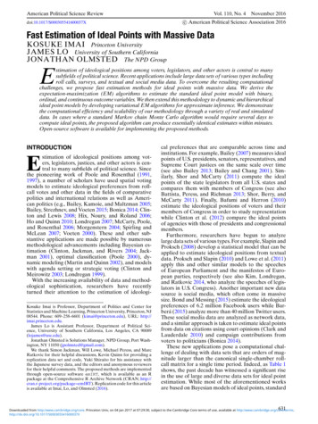
American Political Science ReviewFIGURE 1.Vol. 110, No. 4Comparison of Computational Performance across the MethodsNotes: Each point represents the length of time required to compute estimates where the spacing of time on the vertical axis is basedon the log scale. The proposed EM algorithm, indicated by “EM,” “EM (high precision),” “EM (parallel high precision),” and “EM withBootstrap” is compared with “W-NOMINATE” (Poole et al. 2011), the MCMC algorithm “IDEAL” (Jackman 2012), and the nonparametricoptimal classification estimator “OC” (Poole et al. 2012). The EM algorithm is faster than the other approaches whether focused onpoint estimates or also estimation uncertainty. Algorithms producing uncertainty estimates are labeled in bold, italic type.et al. 2011), and the nonparametric optimal classification estimator implemented as oc() in the R packageoc (Poole et al. 2012). For all roll-call matrices, we restrict attention to just those legislators with at least 25observed votes on nonunanimous bills. In all cases, weassume a single spatial dimension.We caution that the comparison of computationalefficiency presented here is necessarily illustrative. Theperformance of any numerical algorithm may dependon starting values, and no absolute convergence criteria exists for any of the algorithms we examine. Forthe MCMC algorithm, we run the chain for 100,000iterations beyond a burn-in period of 20,000 iterations.Inference is based on a thinned chain where we keepevery 100 draws. While the length of chain and itsthinning interval are within the recommended rangeby Clinton, Jackman, and Rivers (2004), we emphasizethat any convergence criteria used for deciding whento terminate the MCMC algorithm is somewhat arbitrary. The default diffuse priors, specified in ideal()from the R package pscl, are used and propensitiesfor missing votes are not imputed during the dataaugmentation step. In particular, we assume a singledimensional normal prior for all ideal point parameters with a mean of 0 and a variance of 1. For thebill parameters, we assume a two-dimensional normalprior with a mean vector of 0’s and a covariance matrixwith each variance term equal to 25 and no covariance. The standard normalization of ideal points, i.e.,a mean of 0 and a standard deviation of 1, is used forlocal identification. The MCMC algorithm producesmeasures of uncertainty for the parameter estimatesand so we distinguish it from those algorithms whichproduce only point estimates by labeling it in Figure 1with bold, italic typeface.For the proposed EM algorithm, we use randomstarting values for the ideal point and bill parameters. The same prior distributions as the MCMC algorithm are used for all parameters. We terminate theEM algorithm when each block of parameters has acorrelation with the values from the previous iterationlarger than 1 p. With one spatial dimension, we havethree parameter blocks: the bill difficulty parameters,the bill discrimination parameters and the ideal pointparameters. Following Poole and Rosenthal (1997) (seep. 237), we use p 10 2 . We also consider a far morestringent criterion where p 10 6 , requiring parameters to correlate greater than 0.999999. In the followingresults, we focus on the latter “high precision” variant,except in the case of computational performance whereresults for both criteria are presented (labeled “EM”and “EM (high precision),” respectively). The resultsfrom the EM algorithm do not include measures of uncertainty. For this, we include the “EM with Bootstrap”variant which uses 100 parametric bootstrap replicates.To distinguish this algorithm from those which producejust point estimates, it is labeled in Figure 1 with bold,italic typeface.Finally, for W-NOMINATE, we do not includeany additional bootstrap trials for characterizing635Downloaded from http:/www.cambridge.org/core. Princeton Univ, on 04 Jan 2017 at 07:29:30, subject to the Cambridge Core terms of use, available at rg/10.1017/S000305541600037X

Fast Estimation of Ideal Points with Massive Datauncertainty about the parameters, so the results willonly include point estimates. For optimal classification,we use the default setting of oc() in the R packageoc. Because the Bayesian MCMC algorithm is stochastic and the EM algorithm has random starting values,we run each estimator 50 times for any given roll-callmatrix and report the median of each performancemeasurement.We begin by examining the computational performance of the EM algorithm.3 Figure 1 shows the timerequired for the ideal point estimation for each Congressional session in the House (left panel) and theSenate (right panel). Note that the vertical axis is onthe log scale. Although the results are only illustrativefor the aforementioned reasons, it is clear that the EMalgorithm is by far the fastest. For example, for the102nd House of Representatives, the proposed algorithm, denoted by “EM,” takes less than one second tocompute estimates, using the same convergence criteriaas W-NOMINATE. Even with a much more stringentconvergence criteria “EM (high-precision),” the computational time is only six seconds. This contrasts withthe other algorithms, which require much more timefor estimation. Although the direct comparison is difficult, the MCMC algorithm is by far the slowest, takingmore than 2.5 hours. Because the MCMC algorithmproduces standard errors, we contrast the performanceof “IDEAL” with “EM with Bootstrap” and find thatobtaining 100 bootstrap replicates requires just underone minute. Even if more iterations are desired, over10,000 bootstrap iterations could be computed beforeapproaching the time required by the MCMC algorithm.The W-NOMINATE and optimal classification estimators are faster than the MCMC algorithm but takeapproximately one and 2.5 minutes, respectively. Thesemethods do not provide measures of uncertainty, andall of the point-estimate EM variants are over ten timesfaster. Last, the EM algorithm is amenable to parallelization within each of the three update steps. Theopen-source implementation that we provide supportsthis on some platforms (Imai, Lo, and Olmsted 2015).And, the parallelized implementation performs well.For any of these roll-call matrices, using eight processor cores to estimate the parameters instead of just onecore reduces the required timeto completion to aboutone-sixth of the single core time.We next show that the computational gain of theproposed algorithm is achieved without sacrificing thequality of estimates. To do so, we directly compareindividual-level ideal point estimates across the methods. Figure 2 shows, using the 112th Congress, that except for a small number of legislators, the estimatesfrom the proposed EM algorithm are essentially identical to those from the MCMC algorithm (left column)and W-NOMINATE (right column). The within-party3 All computation in this article is completed on a cluster computerrunning Red Hat Linux with multiple 2.67-GHz Intel Xeon X5550processors. Unless otherwise noted, however, the computation isdone utilizing a single processor to emulate the computational performance of our algorithms on a personal computer.November 2016correlation remains high across the plots, indicatingthat a strong agreement among these estimates up toaffine transformation.4 The agreement with the resultsbased on the MCMC algorithm is hardly surprisinggiven that both algorithms are based on the same posterior distribution. The comparability of estimates acrossmethods holds for the other sessions of Congress considered.For a small number of legislators, the deviation between results for the proposed EM algorithm and boththe MCMC algorithm and W-NOMINATE is not negligible. However, this is not a coincidence—it resultsfrom the degree of missing votes associated with eachlegislator.5 The individuals for whom the estimatesdiffer significantly all have no position registered formore than 40% of the possible votes. Examples include President Obama, the late Congressman Donald Payne (Democrat, NJ), and Congressman ThomasMassie (Republican, KY).6 With a small amount ofdata, the estimation of these legislators’ ideal points issensitive to the differences in statistical methods.We also compare the standard errors from the proposed EM algorithm using the parametric bootstrapwith those from the MCMC algorithm. Because theoutput from the MCMC algorithm is rescaled to havea mean of zero and standard deviation of 1, we rescalethe EM estimates to have the same sample moments.This affine transformation is applied to each bootstrapreplicate so that the resulting bootstrap standard errorsare on the same scale as those based on the MCMCalgorithm. Figure 3 does this comparison using the estimates for the 112th House of Representatives. The leftpanel shows that the standard errors based on the EMalgorithm with the bootstrap (the vertical axis) are onlyslightly smaller than those from the MCMC algorithm(the horizontal axis) for most legislators. However, fora few legislators, the standard errors from the EM algorithm are substantially smaller than those from theMCMC algorithm. The right panel of the figure showsthat these legislators have extreme ideological preferences.To further examine the frequentist properties of ourstandard errors based on parametric bootstrap, we conduct a Monte Carlo simulation where roll-call votes are4 The same Pearson correlations between the MCMC algorithm andW-NOMINATE for Republicans and Democrats are, respectively,0.96 and 0.98 in the House. In the Senate, they are 0.99 and 0.98.The Spearman correlations within party between the EM algorithmand the nonparametric optimal classification algorithm are 0.77 and0.77 in the House. They are 0.93 and 0.87 in the Senate. The samewithin-party correlations between OC and the W-NOMINATE andMCMC algorithms range from 0

In the item response theory literature, the EM al-gorithm is used to maximize the marginal likelihood function where ability parameters, i.e., ideal point pa-rameters in the current context, are integrated out (Bock and Aitkin 1981). In the ideal point literature, Bailey(2007)andBaileyandChang(2001)usevariants