WIXLIB

ix. Then click OK to save the changes.Note: The false color SWIR, NIR, Red image is now displayed on the map canvas. Vegetated areas appearin shades of green; areas with exposed soils or impervious surfaces appear in shades of pink and red;water as blue.If the colors still look a little muted, you can adjust the display settings again.4. This time zoom into a part of region that is fully covered by land.5. Now open the style box again (right click on the composite image S Thailand 2008 2010 305 90 composite - in the layer pane Properties Style).i. Under Load min/max values place a check in the box next to Clip extent to canvas.ii. Select Load.iii. Then OK.Remote Sensing for Forest Cover Change Detection11

Now your colors should appear more vibrant. See the image below of my adjusted, zoomed in area.Perhaps this is too much contrast – play around with the settings until you have a display you arepleased with.D. Save your project1. Save your project by clicking on the save icon.2. Save the project in the QGIS Projects file folder in the C:\Change detection directory. Name itIntro to QGIS. You’ll notice the default file extension for QGIS projects is ‘.qgs’.E. Load 2013-2015 composite image and adjust display1. Repeat steps A to D to load the 2013 cloud free composite. SpecifyS Thailand 2013 2015 305 90 Composite.tif as the raster to load.2. After you have the 2013 image loaded and set the display, toggle between the two dates ofimagery by clicking on (and off) the top image layer. Click the box to the left of the layer name inthe Layers Panel.3. Do you see any differences between the images?Exploring forest cover change and sub-settingdataThe study region is in the southern part of Thailand (red box in image below); this region was selectedbecause it exhibits changes in forest cover due to plantation activities. In this section, you will do somepreliminary data exploration to see which areas within the study region have undergone changes inforest cover between 2008 and 2013.Remote Sensing for Forest Cover Change Detection12

A. Investigate areas of forest change in Google Earth Engine (Hansen’sglobal forest data products)1. Open the Google Earth Engine Script by clicking on the link below. This script has been created toload and display forest cover as green, forest loss as red, and forest gain in 4811bc1421fdeb2. If the code window doesn’t automatically display after the site has finished loading, select theShow Code option found in the center of the screen, towards the top and drag it down.3. The script should run when you open the link. Although if it does not, click Run to execute thescript. The script is very simple – it loads the tree cover, loss and gain image into the windowdisplay. Loss appears red, forest gain is blue.Note: if you’d like to learn more about Hansen’s Forest Data Products or examples of additional GoogleEarth Engine scripting exercises, visit the tutorials available here https://developers.google.com/earthengine/tutorial hansen 014. Zoom in and scroll around the region – where do you see changes occurring over time? Also feelfree to look around for changes in your home country.Remote Sensing for Forest Cover Change Detection13

5. Turn the gain layer on and off – you’ll notice that the same pixel can be classified as loss and gain.Why is this?You can also visit the University of Maryland Global Forest Change website, which uses Google EarthEngine to display just the areas of forest loss since 2000. These areas are color coded by the yeardeforestation occurred.6. Open this link in your web browser: 3global-foresti. Zoom into the study region (near Phuket in southern Thailand, see image below).ii. To view the map symbols (city names, roads, etc), you can adjust the transparency of theforest loss layer by sliding the button along the continuum just above the forest loss yearlegend.iii. Where are the most recent, large losses in forest cover located within the study region? Thiswill be the larger blue, red, and orange polygons in the map.Remote Sensing for Forest Cover Change Detection14

B. Add forest loss data and zoom to that areaNext you will load a shapefile in QGIS with some previously identified locations that may haveundergone changes in land cover between the two study dates. You will investigate these areas so thatyou can get a sense of what an area undergoing a land cover transition looks like using a false colorcomposite (SWIR, NIR, and red bands).1. Load the shapefile that marks locations that have likely undergone a transition in land coverbetween the two study dates. From the menu bar select Layer Add Layer Add Vector Layer (orclick on the Add Vector Layer icon on the left hand panel).i. Click Browse and navigate to the following shapefile:C:\Change detection\Data\Shapefiles\Data Exploration\Change Examples.shp.ii. Click Open.2. In the Layers panel, right click on the newly loaded layer, Change Examples, and selectProperties. Note – you can also just double click on the layer in the layer panel to open the LayerProperties dialog.i. Select the Style tag from the left panel.ii. Click on the Simple fill box.iii. Use the dropdown to set the Colors Fill to transparent fill.Remote Sensing for Forest Cover Change Detection15

iv. Set the Colors Border to red.v. Set the Border width to 1.vi. Select OK to close the dialog.Your Layers panel should now look something like the figure below (you may need to drag layers up ordown to replicate the order shown here).3. Right click on the Change Examples layer and select Zoom to Layer.4. The features in this shapefile delineate examples of areas that appear to have a change in landcover between the two time steps.5. Zoom in closer to one of the change example areas.6. Toggle the 2008-2010 layer on and off to compare differences between the two images.Note: These areas appear pink in one time period and green in another. This is due to the relativeincrease in reflectance of the SWIR (displayed red) and relative decrease in NIR reflectance (displayed asgreen) from the removal of vegetation and exposure of soil.Remote Sensing for Forest Cover Change Detection16

Image from 2008-2010 CompositeImage from 2013-2015 CompositeC. (Optional) Explore these areas in Google Earth1. If you have Google Earth installed on your laptop, navigate to the kmz file stored here:C:\Change detection\Data\Shapefiles\Data Exploration2. Double-click the file called Change Examples.kmz.3. This will open up the file of these same areas in Google Earth. You can now explore the changes inland cover using the imagery in Google Earth.i. Scroll the slider along the timeline of available imagery (in the upper left hand corner ofGoogle Earth) to view older imagery.4. The imagery in BING maps is another useful data source to use to explore your study region. BINGdoesn’t include an option to load shapefiles into the interface, but you can scroll around andzoom in to regions manually. You can access the BING imagery with the imagery date informationRemote Sensing for Forest Cover Change Detection17

displayed at this website: http://mvexel.dev.openstreetmap.org/bing/. They provide quite clearimagery around the 2008 time period for this study region.D. Creating a subsetWhen testing new algorithms or forms of analysis, computationally it makes sense to start with animage subset. This makes it faster to repeat the analysis with different parameters or options. You willuse the extent of the example shapefile to clip the cloud free composite images.1. Right click on the Change Examples layer in the layer pane window and select Zoom to Layer.2. With your raster image open in QGIS, go to Raster Extraction Clipper.3. For the Input file choose your 2008-2010 cloud free composite image.4. Save the Output file asC:\Change detection\Data\Composite\imagery subset\2008 draw Subset.tif.5. For the Clipping mode choose “Extent”.6. Now draw on the raster layer the extent you want to subset (hint – trace the extent of the displaywindow to get the region of the change example polygons). If you click and drag with the mouse itwill automatically draw a bounding box. Notice that the XY values will be updated. Click OK to runthe subset.7. Leave the clipper dialog open and browse to your 2013-2015 cloud free composite layer andcreate your subset (remember to change the output name so you don’t overwrite your previoussubset) – because the dialog box is still open you can use the same box region that you drew forthe 2008-2010 image. Click OK to run, and then Close to close the dialog.8. The resulting image subsets load with the blue, green, red bands displayed. Use what you learnedearlier in the exercise to change the display to the SWIR, NIR, red false color composite for eachsubset image.Remote Sensing for Forest Cover Change Detection18

E. Exploring NDVI with a single band gray scale displayVegetation indices can be calculated from multispectral imagery; these indices enhance features ofinterest. The normalized difference vegetation index, NDVI, provides a rough estimate of the abundanceof healthy vegetation and provides a means of monitoring changes in vegetation over time. It remainsthe most well-known and oft-used index to detect live green plant canopies.The NDVI ratio is calculated for each pixel in the image by dividing the difference of the near-infrared(NIR) and red color bands by the sum of the NIR and red color bands. The equation is as follows:𝑁𝐷𝑉𝐼 (𝑁𝐼𝑅 𝑟𝑒𝑑)/(𝑁𝐼𝑅 𝑟𝑒𝑑)There are three NDVI bands included in the Google Earth Engine cloud-free composite output: the 10thpercentile, the median, and the 90th percentile over the composite time range. Including the informationabout the upper and lower values over time is useful when classifying agricultural land – as these areasoften vacillate between high values at the peak of the growing season to low values after harvest.NDVI has already been calculated and included in the cloud free composite image stack from the GoogleEarth Engine script. Bands 7-9 in the cloud free composite are the 10th percentile NDVI value, themedian NDVI value, and the 90th percentile NDVI value. You will explore the median value next.1. Double click on the 2008 draw subset in the layers panel.2. Select the Style tab from the left hand column.i. Next use the drop down box to select Singleband gray as the Render type.ii. Use the drop down box to select Band 08 (this is the median NDVI band) as the Gray band.iii. Set the Contrast enhancement as Stretch to MinMax.iv. Keep the other options set as the default value.v. Click Load to update these settings, the properties dialog should look similar to the followinggraphic on the next page, click OK to apply the changes.Remote Sensing for Forest Cover Change Detection19

3. Do the same for 2013 subset data and explore the change in NDVI values in the polygons withinthe Change Examples.shpYour image should look similar to the graphic on the following page. In this single band gray display, thehigh NDVI values are white and the low values are black. Your min and max values might be littledifferent than the snapshot above because of different extents drawn during extracting.Remote Sensing for Forest Cover Change Detection20

F. Exploring NDVI with a single band pseudo color displaySince NDVI represents how green an area is, change the display to a green color scale.1. Double click on the 2008 draw subset in the layers panel.2. Select the Style tab from the left hand column.i. Next use the drop down box to select Singleband pseudocolor as the Render type.ii. Use the drop down box to select Band 08, the median NDVI band, as the Band (to display).iii. Specify Greens from the dropdown under Generate new color map (ramp).iv. Click Load to update the min/max values.v. Change the Mode to Equal Interval (or another option of interest to you).vi. Click the Classify button.vii. Then Select OK, the properties dialog should look similar to the graphic on the next page.3. Do the same for 2013 subset data and explore the change in NDVI values in the polygons withinthe Change Examples.shp.Remote Sensing for Forest Cover Change Detection21

Now the pixels with a high NDVI value will be displayed as a dark green (refer to image below). You canmore clearly see areas where there is an abundance of vegetation (green areas) and areas with sparsevegetation (white areas).4. Save your project.Remote Sensing for Forest Cover Change Detection22

Exercise 7: Land CoverClassificationIntroductionFor this assignment, the requirement is to make a single-date thematic map of some kind using imageclassification. Learning to do image classification well is extremely important and requires experience.So here is your chance to build some experience.Objectives Create an appropriate list of land cover classes that can be used to create your classificationmap Create regions of interest (ROIs) for your classes that can be used to train a machine learningalgorithm Classify your image using a Random forests classifierProject Set upA. Open your QGIS project1. Start QGIS by clicking on the QGIS shortcut on your desktop2. From the toolbar, go to Project Open. Navigate to the QGIS project you created in the previousexercise (C:\Change detection\QGIS Projects\Intro to QGIS.qgs).3. Save this as a new project in the same folder (C:\Change detection\QGIS Projects\). Name itclassification.qgs.B. Subset imagesSince the size of the image you will be working on is not relevant to learning the land cover classificationconcepts, you will classify a subset of the 2008-2010 cloud free composite image. This will reduceprocessing time and allow you to redo steps more efficiently. You created a subset in Exercise 6,however you will repeat this step to make sure you are working with the same spatial extent. This timeyou will subset using a mask layer, a boundary shapefile that has been provided for you in the Datafolder.1. Sub-set the 2008-2010 cloud free composite.i. Go to Raster Extraction Clipper.ii. Set S Thailand 2008 2010 305 90 Composite.tif as the input file.Remote Sensing for Forest Cover Change Detection23

iii. Set the output file asC:\Change detection\Data\Composite\imagery subset\Subset 2008.tif.iv. Set the Clipping mode to Mask layer.v. Set the Mask layer as Processing Subset (found inC:\Change detection\Data\Shapefiles\Thailand\).vi. Hit OK to execute.vii. Close the Clipper dialog box.C. Display subset1. Use what you learned in Exercise 6 to apply a swir, nir, red (bands 6, 4, 3 in the Landsat cloud freecomposite image) false color composite stretch to the subset image. You might need to also setno data in this step.2. Or if you want to copy the style from the full cloud free composite, right click on the image name(S Thailand 2008 2010 305 90 Composite.tif) under Layers and go to Styles Copy Style.3. To apply this matching stretch to your subset, right click on the Subset 2008 image in the Layerspanel. Select Styles Paste Style.4. Turn the other cloud free composite images off (click on the box to the left of the layer name inthe layers panel).5. Zoom to the extent of the new subset layer by right clicking on the Subset 2008 layer in the Layerpanel and select Zoom to Layer.Define land cover classesThe first thing you need to do is define the legend for the map, or the list of classes to be included inyour map. What classes do you want to map? For this exercise try to keep it simple, but perhaps moreinteresting than just forest and non-forest. 3 to 5 land cover classes might be a good choice.It is also important to have definitions for each of the classes. A lack of clear definitions of the land coverclasses can make the resulting maps difficult for others to use. These will probably be workingdefinitions as you move through the land cover classification process. As you become more familiar withthe landscape, data limitations, and the ability of the land cover classification methods to discriminatesome classes better than others, you will undoubtedly need to update your definitions.Remote Sensing for Forest Cover Change Detection24

A. Defining forest land coverThe image on the following page is an excerpt of text from the Methods and Guidance from the GlobalForest Observations Initiative (GFOI) document that describes the Intergovernmental Panel on ClimateChange (IPCC) 2003 Good Practice Guidance (GPG) forest definition and suggestions to consider whendrafting your forest definition.Remote Sensing for Forest Cover Change Detection25

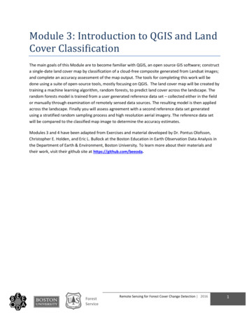
1. Think about what criteria determine if you have a forest vs. another land cover type? An area oftrees that are conserved as a national park, an area that is sustainably logged, and an areamanaged for palm oil all are characterized by tree cover – but they all have very different landuses. Will their spectral signatures differ? Look at the images below – would you characterize allof the images below as forest?Note: The snapshots below are from both high resolution aerial images (left hand side) and the Landsatcloud free image composite (right hand side). During this online training course, you will be mappingland cover across the landscape using the Landsat composite, a moderate resolution data set. You maydevelop definitions based upon your knowledge from the field or from investigating high resolutionimagery. However, when deriving your land cover class definitions, it’s also important to be aware ofhow the definitions relate to the data used to model the land cover. You will continue to explore thisrelationship throughout the exercise.Remote Sensing for Forest Cover Change Detection26

2. Draft a definition for the forest land cover class.Note: the previous series of images are a good illustration of the connections between land use and landcover. You can map land cover with remote sensing data and tools. However most of the time, you areequally, if not more so, interested in land use ̶ for example, reporting the land use, land-use change andforestry activities for REDD . B

Remote Sensing for Forest Cover Change Detection 5 ii. On the left side of the Options dialogue select CRS, which stands for coordinate reference system. iii. In the Default CRS for new projects section click the Select CRS button for the Always start new projects with this CRS field. 2.