Transcription
Excel Formatting: Fonts,Alignments, and Numberstraining@health.ufl.edu
Excel Formatting: Fonts, Alignments, and Numbers1.0 hourA Note About the Ribbon . 3Moving and Duplicating with the Mouse. 3Fill Handle . 3Format Painter . 3Paste. 4Paste Values. 4Other Paste Options . 4Paste Special . 5Formatting Cells . 6Font - Ribbon . 6Font - Format Cells Window . 6Border - Format Cells Window . 7Fill - Format Cells Window . 7Alignment . 8Alignment - Ribbon . 8Alignment - Format Cells Window . 9Numbers. 10Number - Ribbon . 10Number - Format Cells Window . 11Class Exercise . 12Pandora Rose CowartEducation/Training SpecialistUF Health IT TrainingC3-013 CommunicorePO Box 100152Gainesville, FL 32610-0152Updated: 04/28/2020(352) .edu
A Note About the RibbonThe images of Excel in this packet were copied from a wide screen monitor. With the wide screen, the ribbon isstretched across the window and I can see all the buttons. If you are working on a narrower window, Excel willtry to clump the groups together and the layout may look a little different from the ones shown here, but all thebuttons will be there.Here we can see how thefont group is now threebuttons high, and howsome of the buttons likeWrap Text have lost theirtext labels.Moving and Duplicating with the MouseIf you put your mouse over the border of the selected cell(s), you will get the Select Arrow.-Hover over the border and drag (don't let go of the mouse) and a shadow will follow your mouse. Let goin an empty cell and the selected cell will be Moved to the new location. This is an alternative to cut.- Use the Ctrl button while dragging the mouse and you will see a small plus sign added to the shadow.Drag the to an empty cell, be sure to let go of the mouse before the keyboard and Excel will duplicatethe selection instead of moving it. This is an alternative to copy.Fill HandleThe Fill Handle is in the bottom right corner of the selected cell. When you place your mouse over this handle, itchanges from a thick white selection cross, to a thin black cross. Once you see the darker cross, you can click anddrag the cell to fill the original cell's contents into the newly selected cells. The handle allows the mouse to movein a single direction (up, down, left or right). If you want to go in two directions, you must first complete one way,let go of the mouse and then drag again in the second direction.When you use the Fill Handle to pull down a single number or plain text, it will copy the data. This is discussedmore in depth in the Excel Math workshop handout.Format PainterThe Format Painter copies the format of selected cells andapplies the format to the cells you specify. This buttonappropriately shows a paintbrush.This is available in all the Microsoft apps and is one of the most powerfulunderused tools. Click on the object/cell/text with the “good format”, Click on theformat painter, and a paint brush will follow you. Click on the object/cell/text youwant to change and only the format will be pasted.Double-click on this button to use in multiple places.Page 3
PasteWhen you are copying a cell, the paste button has a long list of possibilities. If you click on the clipboard buttonitself, it performs the same action as the very first paste option on its pasting menu.Paste will paste the copied cell contents and formattingFormulas will paste the formulas without formattingFormulas and Number Formatting will paste the copied cell contents andnumber formattingKeep Source Formatting will paste the copied cell contents, number formatting,and cell formatsNo Borders will paste the cell contents and formatting, but no bordersKeep Source Column Widths will paste the cell contents, formatting and cellwidthTranspose will paste a horizontal set of cells into a vertical set of cells, or avertical set of cells into a horizontal set of cellsPaste ValuesPaste Values will paste the unformatted values instead of the formulasPaste values and number formats will paste the raw values instead of the formulas, but with the numberformat from the original cellsValues and Source Formatting will paste the raw values instead of the formulas, but with the numberformat and cell formats from the original cellsOther Paste OptionsFormatting will paste only the formatting from the original cells, not the contents (Format Painter)Paste Link will link the new cell to the old such that any changes to the old data will be made herePaste Picture will create a floating picture based on the copied cellsPaste Linked Picture will create a floating picture based on the copied cells that are linked to the originalvalue so changes made in the original data will be reflected in the picture.Page 4
Paste SpecialThe Paste Special option can be found on the shortcut (right-click) menu, and the Paste dropdown menu (seeprevious page). If this option is grayed out, it means that nothing is currently on the clipboard. If the copieditem is from outside of Excel, you will get a customized screen to paste as text, pictures, or links. If you havecopied from inside of Excel, you will get the following options.- All: paste cell contents and formatting- Formulas: paste the formulas staying true to the absolute and relative references- Values: paste only the raw numbers- Formats: pastes only cell formatting- Comments: pastes comments attached to the cell,but not the data- Validation: pastes data validation rules for thecopied cellsto the paste area- All using Source theme: pastes only theme oforiginal cells- All except borders: pastes cell contents and allformatting except the border lines surrounding theoriginal cells- Column widths: pastes the width of a column (orrange) to another column (or range)- Formulas and number formats: pastes formulas and all number formatting- Values and number formats: paste the raw numbers and number formatting- All merging conditional formats: pastes formulas, formatting and conditional formattingOperation Options- The Paste Special Operation option allows you to specify a mathematical operation.-Example: A1:A2 are copied onto B1:B2, using an Add Operation123A12B24CPANDORA123A12B36COther Options- Skip blanks - Avoids replacing values in your paste area when blank cells occur in the copy area.- Transpose - Changes columns of copied data to rows, and rows of copied data into columns.Paste Link - Links the pasted data to the active worksheet.Page 5
Formatting CellsThe most formatting options are found on the Home Tab. All the options are in the Format Cells window. Thiscontains several tabs to help us format the contents of our spreadsheet. This window can be opened by usingtheMore Options button at the end of the Format, Alignment and Number groups. You can also use theKeyboard Shortcut – Ctrl-1 or choose Format Cells from the right-click shortcut menu.Font - Ribbon123 41.Font – Sets the font of the selected cell(s). Fonts are different waysto show the same letters.2.Font Size – Sets the size of the letters (the font). Larger numbersgive larger fonts. You can type a custom size into this box. Excel willallow you to use the numbers 1 through 409, including half sizes.3.Increase Font – Increases the font to the next Font Size on the list4.Decrease Font – Decreases the font to the next Font Size on the list5.Bold – Makes the selected cell(s) Bold. Shortcut keys are Ctrl-B and Ctrl-2.6.Italic – Makes the selected cell(s) Italicized. Shortcut keys are Ctrl-I and Ctrl-3.7.Underline – Makes the selected cell(s) Underlined. Shortcut keys are Ctrl-U and Ctrl-4. The drop-downarrow lets you choose between single and double underlines.8.Borders – Adds and removes borders for the selected cell(s). The drop-down arrow will provide a longmenu of border possibilities. To get to the dialog box for more control you can choose More Borders 9.Fill Color – Changes the background color of the selected cell(s). By default, the cells have "No Fill"; this isnot the same as a White Background.10. Font Color – Changes the color of the font of the selected cell(s).11. More Options – This button will open the Format Cells dialog window.Font - Format Cells Window- Font sets the font, the shape of the letters of the selected cell(s) or text.- Font Style offers four options. Regular, Italic, Bold,Bold Italic.- Size sets the size of the letters (the font).- Underline places a line under the data.- Color changes the color of the font.- Normal Font will reset the selected cells to thedefault values, which are set in the Excel Options.- Strikethrough places a single line through thevalue in the cell.- Superscript raises and shrinks the selected text,used in text like 3rd and x2. (Superman goes up)- Subscript lowers and shrinks the text, used in textsuch as H2O and HA1C. (Subway goes down)Page 656 78910 11
Border - Format Cells WindowBy default, the gridlines around the cells of your spreadsheet do not print. If you would like them to print, youcan turn them on from the Page Layout Tab; click the Print check box under the Gridlines option.The Font group of the Home Tab has a borders buttonmore customizations, you can come to this window. This button has multiple border options, but forLineYou can choose a line style and a line color that you would like for your border. The line style/color you choosewill not be applied until you choose a Preset or a Border option.PresetsThere are three preset border options: None (no borders), Outline (Top, left, right, bottom borders), and Inside(inner borders). These will be created based on the line style and color selected.BorderThe Border group does more than show a preview of the preset options, it allows you to choose to turn on or offany border (top, middle, bottom, diagonal left, left, center, right, diagonal right). Select the line style and colorand then click within the preview window, or on the actual border button to see the change. To turn off theborder, click on the border or border button again, or choose the None option from the Presets.Fill - Format Cells WindowBy default, the cell background has no color. The Font group of the Home Tab has a fill buttonhas multiple fill options, but for more control, you can open the Format Cells Window.Background ColorThe Background Color shows the same palette of colors we seeon the Home Tab. Click on a color to choose it as your newbackground color.More Colors If the color palette is not sufficient, you can usethe More Colors button. This will give you a honeycomb ofmultiple color options. If you want to go even deeper, you canchoose to Custom build a color.Page 7. This button
Fill Effects The gradient gives the cells more depth of color by showing almost a 3D effect as it changes one color to another.PatternsA pattern allows us to put lines and hashmarks in the background of our cell(s).Along with the pattern that will fill in thebackground, you have the ability to choosethe Pattern Color.AlignmentAlignment - Ribbon123456789 10111.Top Align – Vertically aligns to the top of the cell.2.Middle Align – Vertically aligns to the middle of the cell.3.Bottom Align – Vertically aligns to the bottom of the cell.4.Orientation – Rotates the contents of the cell to thecurrently displayed option.5.Wrap Text – Displays contents on multiple lines within the cell's column width.6.Align Text Left – Horizontally aligns the contents to the left side of the column.7.Center – Horizontally aligns the contents to the center of the cell.8.Align Text Right – Horizontally aligns the contents to the right side of the cell.9.Decrease Indent – Decreases the space between the text and the cell border for Left, Right and Distributedhorizontal alignments.1210. Increase Indent – Increases the space between the text and the cell border for Left, Right and Distributedhorizontal alignments.11. Merge and Center – Joins selected (adjacent) cells into one cell and centers the result. If there is data inmore than one cell, Excel will only keep the information from the upper left cell. The drop-down arrowoffers a few more options, including Merge Cells and Unmerge Cells. Merge and Center will merge the cellsfrom the rows and columns into one large cell. The Merge Across option will merge the cells across thecolumns but not the rows.12. More Options – This button will open the Format Cells dialog window to the Alignment Tab.Page 8
Alignment - Format Cells WindowText AlignmentHorizontal: By default, Excel has a General Horizontal Format, this means that Text is aligned left and numbers arealigned right.- Fill will repeat the contents of the cell as many times as will fit within the width of the column.- Justify keeps the text even on both sides of the cell, as a "full justified" paragraph.- Center Across Selection will center the text in the first cell of across the selection of cells.- Distributed spreads the text out such that text is as evenly distributed as possible. If there is only one word,this option will center the text.- Justify distributed is available when you have chosen a distributed Horizontalalignment. If you choose this option, you will not be able to use an indent with thedistributed text.Vertical: By default, Excel's Vertical alignment is the bottom of the cell. There are fourother options: Top, Center, Justify and Distributed. Top, Center, and Bottom are selfexplanatory.Justified and Distributed vertical alignments will wrap your text so that the contents fitwithin the column width and will place blank space between the lines as necessary tohave the words touching the top and bottom of the cell. If there is only one line of text Justified text will remainat the top of the cell, Distributed in the Middle.The Indent: option only available with the alignments that offer (Indent) in the list.OrientationThese tools allow you rotate your text within 180 degrees, from left side to right side, as well as arranging eachletter into a single column.When you change the orientation, you the borders will follow the slant of the text.For the least amount of distortion, try to stay with the90 , 45 , 0 , -45 and -90 values.Page 9
Text ControlsThe text controls are toggle options. If the box is checked, the option is on; if the box is blank,the option is off. If a light gray check appears in the box, then some cells have the option andsome do not; click once to turn on the option for all selected cells, and again to turn off for allselected cells.- Wrap Text will keep text inside its own cell bycreating multiple lines.- Shrink to fit will reduce the size of the text suchthat it appears smaller when the column is notwide enough to show its true size.- Merge Cells will join the selected (adjacent) cellsinto one cell. If there is data in more than one cell,Excel will only keep the information from theupper left cell.Right to LeftThis option specifies the reading order and alignment for different languages. Text is usually entered to the leftof the cursor; in some languages, it is expected to go to the right of the cursor. This setting will adjust the flow ofdata, if your computer is set to the correct language.Numbers1Number - Ribbon1. Number Format – Allows you to change the way numeric values aredisplayed on the spreadsheet. The drop-down arrow gives you a list of themost common formats, including a More Number Formats option.2.Currency Style – Sets the selected cell(s) to the Currency Style, this stylekeeps the dollar signs on the left side of the cell, and the number on theright side. The drop-down arrow gives you a list of other currency formats,such as the Euro ( ).3.Percent Style – Sets the selected cell(s) to the Percent Style, this style has zero decimal places. Keyboardshortcut - Ctrl-Shift-%. This button can be reset through Cell Styles on the Home Tab.4.Comma Style – Sets the selected cell(s) to the Comma Style, this style has a comma for every thousand andtwo decimal places. This button can be reset through5.Increase Decimal – Increases the number of decimal places showing to the right of the decimal.6.Decrease Decimal – Decreases the number of decimal places showing to the right of the decimal.7.More Options – This button will open the Format Cells dialog window to the Number Tab.Page 10234567
Number - Format Cells WindowMost of the categories have options for you to choose. For example, with a Number category you decide howmany decimal places, if there should be a comma separation at every 1000, and how to display the negativevalues.Dates and Times are numbers, if a date loses its format, Excel will display the numerical representation of thevalue. You can change it back to a date/time format from the General drop-down on the ribbon, or from the Dateor Time categories in the Format Cells window.There are a few Special formats such as include Zip Codes, Phone Numbers and Social Security Numbers. If youtype in 3525551234, and if the cell has a Special "Phone Number" format the cell will display (352) 555-1234.It is possible to create Custom Formats. For example, if you wanted to create a column of UFIDs, you maychoose to create a custom format of 0000-0000. This would ensure that all eight characters are required, andthere is a hyphen in the middle. If we type in 123, we will see 0000-0123.0 – required number# – optional number; – designates format for negative numbers[red] – change color of text redPage 11
Class Exercise-Entering Text (Enter Mode)1. In all lower-case letters, type in cell B2 big city store Notice the status bar will change as soon as you begin to type from READY to ENTER-Editing Text (Edit Mode)1. Double-click to "get inside" cell B2Name BoxCancel/AcceptFormula bar2. Change first letter of each word to uppercase Big City Store3. Press Ctrl-Enter to accept.-Editing Text (Edit Mode)1. Click inside the Formula bar, and notice your status is now Edit. The Cancel and Accept buttons between the name box and the formula bar areavailable when you are in Edit, Enter, and Point modes.-Entering Text in Consecutive Cells1. Type in cell C2 Sale2. Big City Store will be cut off by the Sale. If you are in cell B2, you can look at the Formula barto see the true contents still read "Big City Store"-Adjust Column Widths1. We cannot change the size of one cell, so we need to adjust the column Place your mouse between the column headings B and C and you will see theDrag away from column heading B to make the column widerDrag toward column heading B to make the column skinnier Make it so you can only see Big CityMove back to the resize double arrow and double-click on the line to AutoFitNow, AutoFit Column C-Move the dataset1. Select all the data, move the mouse to the edge of the selection to get the arrows2. Drag the whole block into columns D and E3. Undo the move-Insert Columns1. Right-click on Column Heading B, choose Insert2. Do it again so now data lives in D & E-Formatting Fonts with Home tab,1. Format Font (Cell D2)2. Format Size (Cell D3) Custom Sizing (size 15) Use Increase and Decrease buttons3. Format Bold (D4), Italics (D5) and Underline, Double Underline (D6)4. Format Color (D7)Page 122345678DBig City StoreBig City StoreBig City StoreBig City StoreBig City StoreBig City StoreBig City StoreESaleSaleSaleSaleSaleSaleSale
5. Edit Cell D8 Double-click to "Get Inside" the cell Double-click each word to format Bold: Big, Italicize: City, Underline: Store Notice the text in the formula bar is not formatted-Format Fonts with Format Cells window1. Format Cell E2 using "More" Button Comic Sans, Bold, 14, Double Underline, Green-Use Format Painter1. In cell E2, click on the format painter Dashed Marquee means we are copying Click on cell D2, all changes happen at once2. Try painter again, it turns off Double-click to Keep on, press Esc (escape) to stop3. Change all cells to this font Cell D8 will not format, Delete-Format Column/Row1. Click on Column Letter E to select whole column Change color to Red2. Right-Click on Row Number 4 to select whole row Change color to BlueFormat All1. Click on blank gray square between Column A and Row 1 to select the whole spreadsheet Open the "more" fonts (Format Cells Window) Choose Normal Font (Click the box as many times as needed to show a check mark) Click OK to see the changes--Click on the Plus sign next to Sheet 1 to create Sheet 2-Zoom to 200%-Starting in B2 type:1. B2 - Text2. B3 - 1233. B4 - *2345Text*B12328-AprPage 13
4. B5 - 4/28 The date changes to a different format, but the formula bar shows that Excelassumed the date was for the current year.5. Notice the data is on different sides of the cell (text, number, text, date) Text on the left Numbers & Dates on the right-Alignments with Toolbar1. Select Column B2. From the Alignment Group on the Home tab try the different alignments Left, Center, Right, None (Not left/not center/not right)-Indent1. Bold and Underline B2: Text2. Select B3:B5 Increase Indent Decrease Indent Center Text, Increase Indent, pops back to the left Decrease Indent Right Align Text, Increase indent-Alignments with Menu1. Select all of Column B2. Open the more alignments (format cells) window3. Change the Horizontal option to Fill4. Click OK and see how the cell contents repeat Type into a cell in column B to see the changes Careful of ones like - or - , Excel will think you want an equation and will give youan error message. If you want this pattern, you will need a single quote in front.-Delete Column1. Select Column B, press delete on keyboard2. Type A in cell B2 and Press enter Cell should repeat AAAAAAAAAA Delete on the keyboard erases the cell contents, not the formatting3. Right-click on column B and Choose DELETE Column will be physically removed, along with its formatsCopy from another worksheet1. Turn to Sheet 1 Select the first two Big City Stores Copy2. Turn to Sheet 2 Paste into Cell B2 on Sheet 23. DO NOT ADJUST COLUMN WIDTHS--Try cell alignments to see what happens when cell's not big enough1. Left, center, right, nonePage 14
-Center Across Selection1. Select B2:F22. More Alignments Horizontal: Center Across Selection3. Click OK-Center and Merge Selection1. Select B3:F32. More Alignments Horizontal: Center Text Control: Merge Cells Notice in the Alignment group, there is aMerge and Center button-Copy 2 Big City Stores from Sheet 11. Paste into Cell B6 on Sheet 2-Shrink to fit1. Click in Cell B62. Open format cells box, Alignment tab Text Control Shrink to Fit3. Click OK4. Adjust Column Widths wider, narrower-Wrap Text1. Click in Cell B62. Open format cells window, Alignment Tab Text Control turn off Shrink to Fit Text Control turn on Wrap Text3. Adjust Column Widths so line goes through the Y in CITY Notice in the Alignment group, there is a wrap text button-Forced "Enter"1. Double-Click in Cell B72. Place your cursor in front of the word City3. Press ALT-Enter to force the text to the next line4. Repeat in front of Store5. Adjust column widths6. The bottom of the formula bar can be dragged down to read multiple lines-Vertical alignment1. Adjust the column widths so B6 and B7 match2. Click in Cell C6, type Sale3. Press enter or accept4. In cell C6, change the vertical alignment The Top/Middle/Bottom are above the left/center/right buttonsPage 15
-Text Rotation1. In cell C6, click on the Orientation button to slant text Looks like an angled AB next to align bottom2. Open Format Cells Window to view all ORIENTATION options-Click on the Plus sign next to Sheet 2 to create Sheet 3-Adjust the zoom to 200%-Decimal places1. In cell B2 type: 1.928374650 and press enter This is not the number that shows Move back to that cell and see the true number in the status bar2. Use the Increase Decimal button to show the original number-Too many digits #######1. Resize the column to half its current width2. Notice the number is still in the formula bar, but the cell displays hashtags. This means thecell is too skinny to display the full number.3. Double-click between the column headings to auto fit the cell contents-Format numbers buttons1. Use the Decrease Decimal button until there are no decimals showing2. Click on the Dollar sign button3. Click on the Percentage button4. Click on the Comma style button Edit cell, remove decimal place, Accept5. From the drop-down list in the number group, click General to remove all formatting-Format Special Numbers1. From the corner of the number groupchoose the More button2. Click on the different options Special - SSN Click OKPage 16
-Click on the Plus sign next to Sheet 3 to create Sheet 4-Adjust the zoom to 200%-Fill in data selection1. Select B2:D42. Enter numbers 1-9, press enter to maintain the selection3. Press delete to clear what you typed4. Make sure you still have your nine cells selected Type the number 1 press Ctrl-Enter to accept This should enter a 1 into all nine cells at once5. Center the numbers-Format Background Colors1. While the values are still selected, click on the fill bucket in the Font group2. Open the menu and hover to see a preview of choices3. Hover over the white No gridlines4. Choose No Fill-Add Borders1. Click on the borders button in front of the bucket in the Font group2. Choose ALL BORDERS3. Return to the fill and find one you like4. Click outside the select to see the result-Custom borders1. Select the dataset (B2:D4)2. From the Borders drop-down, choose More Borders Pick a line, pick a color, pick a location to put the lines3. Click Ok and click outside the selection to see the results-Clear Formatting1. Select the entire sheet (space above Row 1, left of Column A)2. In the editing group on the far right of the Home Tab, look for theClear button3. Choose Clear - Clear Formats-Format Fill1. Select the dataset (B2:D4)2. Ctrl- 1, or right-click Format Cells3. Turn to the Fill Page Fill Patterns Fill EffectsPage 17
- Hover over the border and drag (don't let go of the mouse) and a shadow will follow your mouse. Let go in an empty cell and the selected cell will be Moved to the new location. This is an alternative to cut. - Use the Ctrl button while dragging the mouse and you will see a small plus sign added to the shadow. Drag the to an empty cell, be sure to let go of the mouse before the keyboard and .