WIXLIB

This is the author’s peer reviewed, accepted manuscript. However, the online version of record will be different from this version once it has been copyedited and typeset.PLEASE CITE THIS ARTICLE AS DOI:10.1063/1.51218833FIG. 1. Different steps performed by the sample detection software to find an unheated sample ( 1.6 mm) in front of an illuminatedbackground. (a) Image acquired from camera system, (b) Grey-value sums of the 15 px 15 px regions scaled to 8-Bit, (c) Range to detect theborder of the sample based on the lowest sum of grey values, (d) Detected edges identified by highest grey-value gradients in each direction,(e) Calculated centre of levitating sample, (f) Estimated sample-shape based on the calculated radiuspixel at the edge of the sample. The detected points from theexample are highlighted in Fig. 1d.From these four points the coordinates of the samples centreis calculated by averaging horizontal and vertical coordinates,respectively (Fig. 1e). Within the current setup, the centre canbe detected with a spatial resolution of 27 µm in each direction. The uncertainty results from the border detection andcan be estimated to 1.5 px which corresponds to 40 µm.Finally, this algorithm is applied to each of the two cameras. This results in the three dimensional sample position,which is represented by the three coordinates of the samplecentre. These values are transmitted to the feedback controllerto stabilise the sample position. The sample loss informationis forwarded to the sequence control and will trigger feedingin the next sample.In addition the sample radius can be estimated by calculating the average distance between the sample centre and thedetected border points. At present it is used to check the valueagainst a predefined limit to proof the identified object probably is the sample. The estimated sample-shape based on thecalculated radius is shown in Fig. 1f and confirms the detectedsample centre.The detection might be influenced by the relation betweensample position and camera focus, irregular shape and rota-tion of a solid sample, and by light reflections on the surface.All these disturbances can be neglected, for an incandescent,liquid sample close to the centre of the electrode system.For the system used here, the algorithm needs to complete in 5 ms for both cameras. In addition to the steps described above, the image sequences should be stored on a harddisk drive for later analysis and be displayed live on the userscreen. The described algorithm is implemented in NI LabVIEW 2017 using the IMAQdx libraries. The calculated sample position is encoded and sent via a RS232 interface to thefeedback controller.The algorithm is able to perform more than 4000 cycles/susing one core of an Intel i7 processor. It offers enough scopefor future utilisation of faster camera systems and therebyfaster control algorithms and better observation of sample.IV.CONTROL MODELTo implement a suitable controller for stabilising the sample position it is necessary to find a control model for theelectrostatic levitator. For laboratory systems using five controllable and one grounded electrodes a model is describedin Refs. 1 and 19. The ELF facility also uses six electrodes

This is the author’s peer reviewed, accepted manuscript. However, the online version of record will be different from this version once it has been copyedited and typeset.PLEASE CITE THIS ARTICLE AS DOI:10.1063/1.51218834Coulomb’s law. For the resulting acceleration of the sample,the fields of all electrodes can be calculated as the superposition of the four fields. In addition, the calculation of the electrical field needs to consider the image charges on each electrode. For the rod electrodes, the positions of those chargesare inside the electrodes. For a sample position in the originthe superposition of the electrical fields of the image chargesneutralises.The resulting non-linear differential equation, describingthe movement of the charged sample in the electrostatic field,is given in Eq. (2). QEi is the charge of the electrode, εR therelative permittivity, ε0 the vacuum permittivity and r the position vector in the field. a r̈ FIG. 2. Electrode system of the microgravity electrostatic levitatorwith four separate electrodes to control the three-dimensional position of the levitated sample24 . In the current setup, the distance between the centres of the electrodes is 10 mm and the electrodes havea diameter of 3 mm.arranged orthogonally17,23 . In all those cases the control system can be separated into three one-dimensional problems. InRef. 14 a tetrahedral electrode-system using four controllersis presented. This setup requires a conversion between theCartesian camera-coordinates and the electrode positions. Allmentioned configurations cannot offer accessibility from allsides to the levitation area.A new electrode system24 , using only four electrodes wasdeveloped to meet the environmental conditions of microgravity. The setup allows the direct usage of the Cartesian cameracoordinates for the control system and offers full accessibility to the levitating sample from all six planes. In order togain stable control of the levitating sample inside this electrode system, a new control model needs to be formulated.The outputs of the system model are the three spatial coordinates x, y, z in mm of the sample position. The inputs arethe voltages of the four electrodes UX0Z0 ,UX1Z0 ,UY 0Z1 ,UY 1Z1in V. Fig. 2 shows the geometric conditions in the electrodesystem model with a sample in the origin.The sample is considered as a point with an electricalcharge of qP in A s and a mass m in kg. If it is exposed tothe electrical field E of a point electrode, motion results fromelectrostatic, inertial, gravitational, and frictional forces.Under microgravity conditions and using a vacuum chamber, the gravitational and frictional forces can be neglected.The acceleration a of the sample can be calculated by Eq. (1). a qP Em4QEi riqP 4πε0 εR m i 1 ri 3(2)Eq. (2) uses the charges of the electrodes as model input.Using high-voltage amplifiers, it is only possible to controlthe potential of the electrodes but not the charges. Both parameters correlate linearly.The controller is needed to stabilise the sample positionin the centre position between the electrodes. It meansthe setpoint for the desired position is constant. Considering Eq. (2) and a possible steady gravitational force, theelectric charges of the electrodes need to be constant toachieve an unstable equilibrium. A combination of sample position x0 , y0 , z0 and the voltages on the electrodesU0,X0Z0 ,U0,X1Z0 ,U0,Y 0Z1 ,U0,Y 1Z1 is defined as the operatingpoint of the system. In ideal circumstances it is identical tothe unstable equilibrium. For controller design, the nonlinearmodel should be linearised around this point using first orderTaylor series.The resulting linear model for the sample movementby the electrostatic field is given in Eq. (3).Inthese equations the positions x, y, z and the voltages uX0Z0 , uX1Z0 , uY 0Z1 , uY 1Z1 describe the deviations fromthe predefined operating point. The directions x, y and z aswell as the indices of the potentials u refer to Fig. 2. P and Kare linear factors resulting from constants in Eq. (2) and fromthe linearisation. ẍ Px x Kx ( uX0Z0 uX1Z0 ) ÿ Py y Ky ( uY 0Z1 uY 1Z1 ) z̈ Pz z Kz (( uX0Z0 uX1Z0 ) ( uY 0Z1 uY 1Z1 ))(3)The linearisation shows good approximation in the range of 2 mm around the operating point along each axis. Considering the radius of the used samples from 0.6 mm to 1.1 mmit is enough to calculate a controller for stabilising the sampleposition.(1)For the controller model, the electrodes are considered aspoint charges with position in the middle of each rod electrode. The electric field of each electrode can be calculated byV.CONTROLLERThe model developed in the previous section is the basis forthe controller implementation. In Ref. 19 a gain scheduling

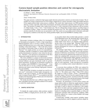
This is the author’s peer reviewed, accepted manuscript. However, the online version of record will be different from this version once it has been copyedited and typeset.PLEASE CITE THIS ARTICLE AS DOI:10.1063/1.51218835controller for electrostatic levitator on ground is presented.The controller uses an estimation of the sample charge toadapt the control parameters. This estimation needs a constant gravitational force and is not applicable for microgravity conditions. In addition, the existing electrostatic levitationfacilities described in Refs. 15 and 19 use five or six controllable electrodes and for each axis the electrodes are separated.In the specific microgravity setup24 , only four electrodes arepresent. The developed controller needs to share electrodesto control the sample position in the three axes as shown inEq. (3).According to the unstable, linear model presented inEq. (3), a PID controller for each axis is used for the microgravity electrostatic levitator.The differential part is necessary to obtain a stable closedloop feedback control. The levitating sample needs to be inthe middle of the electrode system as shown in Fig. 2 to allowproper heating and temperature measurement. Therefore, anintegral action in the controller is required.With Eq. (3) and the standard PID-controller equation, theclosed control loop can be calculated. Studies with a swinging sample were used to adjust the unknown parameters ofthe linearised model. In combination with the closed loopequation, the controller parameters can be calculated to gainstability and robustness for the sample positioning. The outputs of the three PID controllers are three differential voltages ux , uy and uz . To calculate the output of each highvoltage-amplifier, they have to be portioned among the fourelectrodes and the operating point needs to be added. Thecorresponding equations are presented in Eq. 4.UX0Z0 U0,X0Z0 0.5 ux 0.25 uzUX1Z0 U0,X1Z0 0.5 ux 0.25 uzUY 0Z1 U0,Y 0Z1 0.5 uy 0.25 uzUY 1Z1 U0,Y 1Z1 0.5 uy 0.25 uz(4)The control algorithm is implemented on a National Instruments CompactRIO system with a Virtex-5 LX 110 FPGA(Field Programmable Gate Array) running at 500 Hz. Thecontrol software is written in NI LabVIEW using the FPGAToolbox. The sample position is received by the FPGA fromthe detection computer as a four byte array via serial interface.In this array, three bytes represent the sample position in thedetection range of 240 px for three axes. The fourth byte indicates the frame end and includes information about statusof background illumination and possibly lost samples. If nosample is detected, the controller uses the positions from theprevious iteration.To gain the most current position, the last four bytes in thebuffer are analysed. The controller runs faster than the sample detection cameras. If the camera was not able to send anew sample position, the controller continues with the previous one. The received positions in pixels are converted todeviations from the centre of the electrode system in mm.The FPGA calculates the potential differences for each ofthe three axes using the time discrete version of the PIDcontroller. Then outputs for the four amplifiers are calculated.In the next step, the voltage is limited to the respective maxi-mum output of the amplifiers. The last step is the calculationof the control voltage by dividing the limited output by thegain factor.The analogue voltage output is realised using the high speedNational Instruments C-series module 9263 with an accuracyof 16 bit. In addition, the measured positions and the calculated output are transferred to the host system for data loggingusing FPGA FIFOs. After receiving a predefined number ofconsecutive information on a lost sample, the host system isstarting to load and process the next one.VI.PERFORMANCE TESTSFor microgravity experiments, all electrodes are operatingin the same voltage range of 3 kV. For ground experiments,the two amplifiers connected to the bottom electrodes are replaced to offer up to 20 kV for lifting the sample. Additionally, the sample release method differs between microgravityand laboratory. In microgravity, the sample is hold betweentwo rods and released by pulling both rods apart (see Fig. 3).It takes up to 3 frames for the rods to move out of the sample detection area. During this time, the rods may disturb thesample detection and the position controller cannot be used.Assuming a free fall, in those 15 ms, the sample would movemore than 1 mm, which is one third of the levitation area. Thecontroller directly needs to apply a high voltage on the lowerelectrodes to catch the falling sample. If the sample is not sufficiently charged it will get lost. Tests showed, that levitationstarting with a sample placed on the lower rod (like done inRef. 25) are much more reliable on ground. In microgravity,the initial sample movement depends only on small residualaccelerations resulting from the vehicle or the movement ofthe rods. Under this condition, there is enough time for thecontroller to capture it.Multiple tests were performed on ground to obtain the desired levitation stability. The experiments showed that thecharge of the sample is not reproducible. It depends on samplematerial, surface, contact between sample and rod and otherparameters which are not directly accessible. So the parameterqP , used to build the model in Eq. (2), is unknown. In laboratory environment an in-loop estimation of the sample chargebased on the potential difference along the gravitational axiscould be used19 . This method is not possible in microgravity. High speed camera recordings of the levitation process onground show that the sample bounces multiple times on theelectrode before it finally lifts off. If the sample is not chargedsufficiently, it will fall back onto the electrode and recharge.After successful positioning tests in laboratory, the systemwas tested under microgravity conditions at the ZARM droptower in Bremen. Due to the different sample release method(Fig. 3), multiple contacts of the sample with the electrodecannot be performed. As a result, the initial charge of the released sample varies between the experiments. In experimentsat the drop tower, it could be observed that even applying themaximum field strength, some samples were not influencedby the electrostatic field.For samples with sufficient charge, the sample detection

This is the author’s peer reviewed, accepted manuscript. However, the online version of record will be different from this version once it has been copyedited and typeset.PLEASE CITE THIS ARTICLE AS DOI:10.1063/1.51218836the 28th DLR parabolic flight campaign. Compared to thedrop tower, residual accelerations are much higher (approx.10 2 g)27 . During the campaign, levitation was performed onpreheated Zr64 Ni36 ( 1.4 mm, m 10 mg) and La80 Cu20( 1.4 mm, m 9 mg) samples.In 2017, the experiment was onboard the MAPHEUS 6sounding rocket. The sample detection worked as expectedbut due to a failure of one high voltage amplifier, offering onlylimited voltage output, only a few samples could be levitatedsuccessfully.VII.FIG. 3. Sample release mechanism in microgravity performed duringa parabolic flightalgorithm and controller showed good performance. Fig. 4shows a successful levitation process of a Zr64 Ni36 samplewith a diameter of 1.9 mm and a mass of 25 mg in a droptower. The three coordinates of the sample and the associatedelectrode potentials are depicted. For microgravity conditions,the operating point was set to 1500 V for all electrodes andthe output was limited to the range from 0 kV to 3 kV. Thesample was released at 0 s and at 4.1 s, the capsule with theexperiment reached the deceleration chamber and the microgravity phase ended. The sample was not heated because ofthe short drop time of 4.74 s.During the release, an initial speed in direction of x wasmeasured on the sample. The recovery time is about 1.5 s.After 3 s, only small, unavoidable position changes due to thesystem instability remain. The overall control stability was 50 µm for all axes. It includes a minor detection error resulting from the rotation of the not completely spherical sample.The voltage spikes in Fig. 4 result from the differential partof the PID-controller. Due to the sample detection, the position can only change in discrete steps of 27 µm. With thecontroller parameters used during the experiment, a voltagechange of approx. 600 V is calculated and portioned amongthe electrodes, as given in Eq. 4.Even under small residual accelerations (in the order of10 6 g)26 , the full field strength of 3 kV was reached duringthe levitation.Further developments focused on obtaining a higher initialsurface charge. Better results were achieved by improvingthe contact between the sample and the rod and by preheating. Additionally the limitations of the electrode potentialswere removed to offer a field strength of 6 kV and the delay between sample release and controller reaction was minimized. Those improvements were successfully tested onCONCLUSION AND OUTLOOKThis paper describes a fast and reliable way to measureand control the sample position for a microgravity electrostatic levitator. Conventionally used PSD-based sampledetection systems turned out to be unreliable in harsh environments. Hence, for microgravity electrostatic levitation, aCCD-camera-based system is used and proved to offer morereliable results.In order to determine the 3d sample position from the acquired images, a sample detection algorithm was developed.It is designed to identify fast moving single spherical objects.While other less specialised algorithms do not meet the performance requirements, the presented one is by now approximately twenty times faster than the current image acquisitionhardware. It offers the possibility to use camera systems withhigher frame rates or resolution in future developments.Three PID c

flights or on sounding rockets manual adjustment is not pos-sible. To overcome those problems the PSDs were replaced by two CCD (charge coupled device) cameras. First experiences with CCD-based measurement of sample position are given in Ref. 14. The authors used a 50px 50px CCD to detect the sample in a range of 10mm 10mm. A threshold black