Transcription
Stress testing frameworkQuantitative approachesFinancial Risk ManagementLecture 11. Stress Testing and Scenario AnalysisThierry Roncalli?University of Paris-SaclayNovember 2020Thierry RoncalliFinancial Risk Management (Lecture 11)1 / 45
Stress testing frameworkQuantitative approachesGeneral information1234567Thierry RoncalliOverviewThe objective of this course is to understand the theoretical andpractical aspects of risk managementPrerequisitesM1 Finance or equivalentECTS4KeywordsFinance, Risk Management, Applied Mathematics, StatisticsHoursLectures: 36h, Training sessions: 15h, HomeWork: 30hEvaluationThere will be a final three-hour exam, which is made up of questionsand exercisesCourse ent.htmlFinancial Risk Management (Lecture 11)2 / 45
Stress testing frameworkQuantitative approachesObjective of the courseThe objective of the course is twofold:Thierry Roncalli1knowing and understanding the financial regulation (banking andothers) and the international standards (especially the Basel Accords)2being proficient in risk measurement, including the mathematicaltools and risk modelsFinancial Risk Management (Lecture 11)3 / 45
Stress testing frameworkQuantitative approachesClass scheduleCourse sessionsSeptember 11 (6 hours, AM PM)September 18 (6 hours, AM PM)September 25 (6 hours, AM PM)October 2 (6 hours, AM PM)Tutorial sessionsOctober 10 (3 hours, AM)October 16 (3 hours, AM)November 13 (3 hours, AM)December 4 (6 hours, AM PM)November 20 (6 hours, AM PM)November 27 (6 hours, AM PM)Class times: Fridays 9:00am-12:00pm, 1:00pm–4:00pm, University of EvryThierry RoncalliFinancial Risk Management (Lecture 11)4 / 45
Stress testing frameworkQuantitative approachesAgendaLecture 1: Introduction to Financial Risk ManagementLecture 2: Market RiskLecture 3: Credit RiskLecture 4: Counterparty Credit Risk and Collateral RiskLecture 5: Operational RiskLecture 6: Liquidity RiskLecture 7: Asset Liability Management RiskLecture 8: Model RiskLecture 9: Copulas and Extreme Value TheoryLecture 10: Monte Carlo Simulation MethodsLecture 11: Stress Testing and Scenario AnalysisLecture 12: Credit Scoring ModelsThierry RoncalliFinancial Risk Management (Lecture 11)5 / 45
Stress testing frameworkQuantitative approachesTextbookRoncalli, T. (2020), Handbook of Financial Risk Management,Chapman & Hall/CRC Financial Mathematics Series.Thierry RoncalliFinancial Risk Management (Lecture 11)6 / 45
Stress testing frameworkQuantitative approachesAdditional materialsSlides, tutorial exercises and past exams can be downloaded at thefollowing ment.htmlSolutions of exercises can be found in the companion book, which canbe downloaded at the following mentBook.htmlThierry RoncalliFinancial Risk Management (Lecture 11)7 / 45
Stress testing frameworkQuantitative approachesAgendaLecture 1: Introduction to Financial Risk ManagementLecture 2: Market RiskLecture 3: Credit RiskLecture 4: Counterparty Credit Risk and Collateral RiskLecture 5: Operational RiskLecture 6: Liquidity RiskLecture 7: Asset Liability Management RiskLecture 8: Model RiskLecture 9: Copulas and Extreme Value TheoryLecture 10: Monte Carlo Simulation MethodsLecture 11: Stress Testing and Scenario AnalysisLecture 12: Credit Scoring ModelsThierry RoncalliFinancial Risk Management (Lecture 11)8 / 45
Stress testing frameworkQuantitative approachesDefinitionMethodologies“Stress testing is now a critical element of risk management forbanks and a core tool for banking supervisors and macroprudentialauthorities” (BCBS, 2017, page 5).Thierry RoncalliFinancial Risk Management (Lecture 11)9 / 45
Stress testing frameworkQuantitative approachesDefinitionMethodologiesGeneral objectiveIf we consider a trading book portfolio, we recall that:Ls (w ) Pt (w ) g (F1,s , . . . , Fm,s ; w )In the case of a stress testing program, we have:Lstress (w ) Pt (w ) g (F1,stress , . . . , Fm,stress ; w )where (F1,stress , . . . , Fm,stress ) is the stress scenarioThierry RoncalliFinancial Risk Management (Lecture 11)10 / 45
Stress testing frameworkQuantitative approachesDefinitionMethodologiesScenario design and risk factors2004 FSAP stress scenarios applied to the French banking systemF1 flattening of the yield curve due to an increase in interest rates:increase of 150 basis points (bp) in overnight rates, increase of 50 bpin 10-year rates, with interpolation for intermediate maturitiesF5 share price decline of 30% in all stock marketsF9 flattening of the yield curve (increase of 150 basis points in overnightrates, increase of 50 bp in 10-year rates) together with a 30% drop instock marketsM2 increase to USD 40 in the price per barrel of Brent crude for two years(an increase of 48% compared with USD 27 per barrel in the baselinecase), without any reaction from the central bank; the increase in theprice of oil leads to an increase in the general rate of inflation and adecline in economic activity in France together with a drop in globaldemandThierry RoncalliFinancial Risk Management (Lecture 11)11 / 45
Stress testing frameworkQuantitative approachesDefinitionMethodologiesScenario design and risk factorsClassificationThierry Roncalli1historical scenario: “a stress test scenario that aims at replicating thechanges in risk factor shocks that took place in an actual pastepisode”2hypothetical scenario: “a stress test scenario consisting of ahypothetical set of risk factor changes, which does not aim toreplicate a historical episode of distress”3macroeconomic scenario: “a stress test that implements a linkbetween stressed macroeconomic factors [.] and the financialsustainability of either a single financial institution or the entirefinancial system”4liquidity scenario: “a liquidity stress test is the process of assessingthe impact of an adverse scenario on institution’s cash flows as well ason the availability of funding sources, and on market prices of liquidassets”Financial Risk Management (Lecture 11)12 / 45
Stress testing frameworkQuantitative approachesDefinitionMethodologiesScenario design and risk factorsFigure: 2017 DFAST supervisory scenarios: Domestic variablesThierry RoncalliFinancial Risk Management (Lecture 11)13 / 45
Stress testing frameworkQuantitative approachesDefinitionMethodologiesScenario design and risk factorsFigure: 2017 DFAST supervisory scenarios: International variablesThierry RoncalliFinancial Risk Management (Lecture 11)14 / 45
Stress testing frameworkQuantitative approachesDefinitionMethodologiesFirm-specific versus supervisory stress testingExamples of hard trading limits:Unobservable parameters (e.g. correlations of basket options)Less liquid assetsExamples of supervisory stress testing:Financial sector assessment program (FSAP)Dodd-Frank Act stress test (DFAST)EU-wide stress testingThierry RoncalliFinancial Risk Management (Lecture 11)15 / 45
Stress testing frameworkQuantitative approachesDefinitionMethodologiesHistorical approachTable: Worst historical scenarios of the S&P 500 indexSc.12345Sc.12345Thierry 061962-06-22 20.47 9.03 8.93 8.79 8.28 37.66 31.95 27.29 26.89 009-03-09 27.33 18.34 17.43 13.85 13.01 41.11 30.17 28.59 27.55 970-05-26Financial Risk Management (Lecture 11) 30.02 28.89 22.11 19.65 16.89 46.64 34.33 31.29 26.59 25.4516 / 45
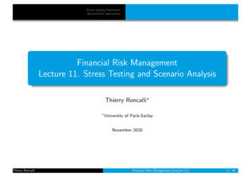
Stress testing frameworkQuantitative approachesDefinitionMethodologiesMacro-economic approachExogenousShockModelRiskFactorsFigure: Macroeconomic approach of stress testingThierry RoncalliFinancial Risk Management (Lecture 11)17 / 45
Stress testing frameworkQuantitative approachesDefinitionMethodologiesMacro-economic approachE1.ModelRiskFactorsEi.EnFigure: Feedback effects in stress testing modelsThierry RoncalliFinancial Risk Management (Lecture 11)18 / 45
Stress testing frameworkQuantitative approachesDefinitionMethodologiesProbabilistic approachAt first approximation, a stress scenario can be seen as an extremequantile or value-at-risk we can use EVT (extreme value theory)Thierry RoncalliFinancial Risk Management (Lecture 11)19 / 45
Stress testing frameworkQuantitative approachesUnivariate stress scenariosJoint stress scenariosConditional stress scenariosReverse stress testingUnivariate stress scenariosLet X be the random variable that produces the stress scenario S (X ).If X F and the relationship between L (w ) and X is decreasing, wehave:Pr {X S (X )} F (S (X ))Given a stress scenario S (X ), we deduce its severity:α F (S (X ))We can also compute the stressed value given the probability ofoccurrence α:S (X ) F 1 (α)α 0 (6 value-at-risk)Thierry RoncalliFinancial Risk Management (Lecture 11)20 / 45
Stress testing frameworkQuantitative approachesUnivariate stress scenariosJoint stress scenariosConditional stress scenariosReverse stress testingUnivariate stress scenariosReturn timeWe have T α 1 and α T 1We reiterate that:T α 1 n · (1 αGEV ) 1where n is the length of the block maximaTable: Probability (in %) associated to the return period T in yearsReturn periodDailyWeeklyMonthly1 αGEVThierry 41670.3846300.01280.06410.27780.2564Financial Risk Management (Lecture 11)500.00770.03850.16670.153821 / 45
Stress testing frameworkQuantitative approachesUnivariate stress scenariosJoint stress scenariosConditional stress scenariosReverse stress testingUnivariate stress scenariosTable: GEV parameter estimates (in %) of MSCI USA and MSCI EMU indicesParameterµσξThierry RoncalliLong positionMSCI USA MSCI EMU1.2421.5720.7200.84419.36321.603Short positionMSCI USA MSCI EMU1.3171.5990.5770.73026.34126.494Financial Risk Management (Lecture 11)22 / 45
Stress testing frameworkQuantitative approachesUnivariate stress scenariosJoint stress scenariosConditional stress scenariosReverse stress testingUnivariate stress scenariosTable: Stress scenarios (in %) of MSCI USA and MSCI EMU indicesYear510255075100ExtremestatisticT?Thierry RoncalliLong positionMSCI USA MSCI EMU 5.86 7.27 7.06 8.83 8.92 11.29 10.56 13.49 11.62 14.94 12.43 16.05Short positionMSCI USA MSCI .5917.26 9.51 10.9411.0410.8732.4922.2447.8720.03Financial Risk Management (Lecture 11)23 / 45
Stress testing frameworkQuantitative approachesUnivariate stress scenariosJoint stress scenariosConditional stress scenariosReverse stress testingUnivariate stress scenariosFigure: Stress scenarios (in %) of MSCI USA and MSCI EMU indicesThierry RoncalliFinancial Risk Management (Lecture 11)24 / 45
Stress testing frameworkQuantitative approachesUnivariate stress scenariosJoint stress scenariosConditional stress scenariosReverse stress testingBivariate stress scenariosWe note p Pr {Xn:n,1 S (X1 ) , Xn:n,2 S (X2 )} the jointprobability of stress scenarios (S (X1 ) , S (X2 ))We have:p 1 F1 (S (X1 )) F2 (S (X2 )) C (F1 (S (X1 )) , F2 (S (X2 ))) C̄ (F1 (S (X1 )) , F2 (S (X2 )))where C̄ (u1 , u2 ) 1 u1 u2 C (u1 , u2 )We deduce that the failure area is represented by:non(S (X1 ) , S (X2 )) R2 C̄ (F1 (S (X1 )) , F2 (S (X2 ))) TWe have:nT C̄ (F1 (S (X1 )) , F2 (S (X2 )))and:max (T1 , T2 ) T nT1 T2Thierry RoncalliFinancial Risk Management (Lecture 11)25 / 45
Stress testing frameworkQuantitative approachesUnivariate stress scenariosJoint stress scenariosConditional stress scenariosReverse stress testingBivariate stress scenariosFigure: Failure area of MSCI USA and MSCI EMU indices (blockwisedependence)Thierry RoncalliFinancial Risk Management (Lecture 11)26 / 45
Stress testing frameworkQuantitative approachesUnivariate stress scenariosJoint stress scenariosConditional stress scenariosReverse stress testingBivariate stress scenariosFigure: Failure area of MSCI USA and MSCI EMU indices (daily dependence)Thierry RoncalliFinancial Risk Management (Lecture 11)27 / 45
Stress testing frameworkQuantitative approachesUnivariate stress scenariosJoint stress scenariosConditional stress scenariosReverse stress testingMultivariate stress scenarios C̄ has a compliacted expression (see HFRM, Section 14.2.2.2, page 908)Thierry RoncalliFinancial Risk Management (Lecture 11)28 / 45
Stress testing frameworkQuantitative approachesUnivariate stress scenariosJoint stress scenariosConditional stress scenariosReverse stress testingThe conditional expectation solutionGiven a joint stress scenario S (X ) (S (X1 ) , . . . , S (Xn )), the conditionalstress scenario of Y is:S (Y ) E [Yt Xt (S (X1 ) , . . . , S (Xn ))]nX β0 βi S (Xi )i 1Thierry RoncalliFinancial Risk Management (Lecture 11)29 / 45
Univariate stress scenariosJoint stress scenariosConditional stress scenariosReverse stress testingStress testing frameworkQuantitative approachesThe conditional expectation solutionLogit transformationWe use the following transformation: YtZt ln1 YtWe have:Yt exp (Zt )1 h (Zt )1 exp (Zt )1 exp ( Zt )where h (z) is the logit transformationWe deduce that:Z E [Yt Xt (x1 , . . . , xn )] h β0 Thierry RoncallinX!βi Xi,t ωi 1Financial Risk Management (Lecture 11)1 ω φdωσσ30 / 45
Stress testing frameworkQuantitative approachesUnivariate stress scenariosJoint stress scenariosConditional stress scenariosReverse stress testingThe conditional expectation solutionExampleWe assume that the probability of default PDt at time t is explainedby the following linear regression model: PDtln 2.5 5gt 3πt 2ut εt1 PDtwhere εt N (0, 0.25), gt is the growth rate of the GDP, πt is theinflation rate, and ut is the unemployment rateThe baseline scenario is defined by gt 2%, πt 2% and ut 5%The stress scenario is equal to gt 8%, πt 5% and ut 10%Thierry RoncalliFinancial Risk Management (Lecture 11)31 / 45
Stress testing frameworkQuantitative approachesUnivariate stress scenariosJoint stress scenariosConditional stress scenariosReverse stress testingThe conditional expectation solutionFigure: Probability density function of PDtThierry RoncalliFinancial Risk Management (Lecture 11)32 / 45
Stress testing frameworkQuantitative approachesUnivariate stress scenariosJoint stress scenariosConditional stress scenariosReverse stress testingThe conditional expectation solution The conditional expectation is equal to 7.90% for the baseline scenarioand 12.36% for the stress scenario The figure of 7.90% can be interpreted as the long-run (orunconditional) probability of default that is used in the IRB formula (i.e.Pillar I) The figure of 12.36% may be used in Pillar IIThierry RoncalliFinancial Risk Management (Lecture 11)33 / 45
Stress testing frameworkQuantitative approachesUnivariate stress scenariosJoint stress scenariosConditional stress scenariosReverse stress testingThe conditional expectation solutionFigure: Relationship between the macroeconomic variables and PDtThierry RoncalliFinancial Risk Management (Lecture 11)34 / 45
Stress testing frameworkQuantitative approachesUnivariate stress scenariosJoint stress scenariosConditional stress scenariosReverse stress testingThe conditional expectation solutionTable: Stress scenario of the probability of defaultt0123456789101112Thierry Roncalligt2.00 6.00 7.00 9.00 7.00 7.00 6.00 4.00 2.00 0.009.008.007.006.006.006.00E [PDt S (X .827.147.14q90% (S (X 6812.6811.6011.60Financial Risk Management (Lecture 11)35 / 45
Stress testing frameworkQuantitative approachesUnivariate stress scenariosJoint stress scenariosConditional stress scenariosReverse stress testingThe conditional quantile solutionWe could also define the conditional stress scenario S (Y ) qα (S (X )) asthe solution of the quantile regression:Pr {Yt qα (S) Xt S} αThe solution is given by:S (Y ) qα (S) F 1C 1y2 1 (Fx (S (X )) , α) See HFRM, Section 14.2.3.2, pages 912-915Thierry RoncalliFinancial Risk Management (Lecture 11)36 / 45
Stress testing frameworkQuantitative approachesUnivariate stress scenariosJoint stress scenariosConditional stress scenariosReverse stress testingReverse stress testingReverse stress test “means an institution stress test that starts from theidentification of the pre-defined outcome (e.g. points at which aninstitution business model becomes unviable, or at which the institutioncan be considered as failing or likely to fail) and then explores scenariosand circumstances that might cause this to occur ”In stress testing, extreme scenarios of risk factors are used to test theviability of the bank: D 0 if S (L (w )) C(S (F1 ) , . . . , S (Fm )) S (L (w )) D 1 otherwiseIn reverse stress testing, extreme scenarios of risk factors are deducedfrom the bankruptcy scenario:D 1 RS (L (w )) (RS (F1 ) , . . . , RS (Fm ))Thierry RoncalliFinancial Risk Management (Lecture 11)37 / 45
Stress testing frameworkQuantitative approachesUnivariate stress scenariosJoint stress scenariosConditional stress scenariosReverse stress testingReverse stress testingWe recall that:L (w ) (F1 , . . . , Fm ; w )The reverse stress scenario RS is the set of risk factors that corresponds tothe stressed loss RS (L (w )):RS {(RS (F1 ) , . . . , RS (Fm )) : (S (F1 ) , . . . , S (Fm ) ; w ) RS (L (w ))} Not a unique solutionMathematical solutionWe can use the following optimization program(RS (F1 ) , . . . , RS (Fm )) arg max ln f (F1 , . . . , Fm )s.t. (S (F1 ) , . . . , S (Fm ) ; w ) RS (L (w ))where f (x1 , . . . , xm ) is the probability density function of the risk factors(F1 , . . . , Fm )Thierry RoncalliFinancial Risk Management (Lecture 11)38 / 45
Stress testing frameworkQuantitative approachesUnivariate stress scenariosJoint stress scenariosConditional stress scenariosReverse stress testingReverse stress testingWe assume that F N (µF , ΣF ) and L (w ) optimization problem becomes:Pmj 1wj Fj w F. The1 RS (F) arg min (F µF ) Σ 1F (F µF )2s.t. w F RS (L (w ))The Lagrange function is: 1 1 L (F; λ) (F µF ) ΣF (F µF ) λ w F RS (L (w ))2The first-order condition is Σ 1F (F µF ) λw 0. It follows that F µF λΣF w , w F wµ λwΣF w ,F λ RS (L (w )) w µF /w ΣF w and: ΣF w RS (F) µF RS (L (w )) w µFw ΣF wThierry RoncalliFinancial Risk Management (Lecture 11)39 / 45
Stress testing frameworkQuantitative approachesUnivariate stress scenariosJoint stress scenariosConditional stress scenariosReverse stress testingReverse stress testingAnother approach for solving the inverse problem is to consider the jointdistribution of F and L (w ): µFΣFΣF wF N,L (w )w µFw ΣF w ΣF wThe conditional distribution of F given L (w ) RS (L (w )) is Gaussian: F L (w ) RS (L (w )) N µF L(w ) , ΣF L(w )We know that the maximum of the probability density function of themultivariate normal distribution is reached when the random vector isexactly equal to the mean. We deduce that:RS (F) µF L(w )Thierry Roncalli ΣF w RS (L (w )) w µF µF w ΣF wFinancial Risk Management (Lecture 11)40 / 45
Stress testing frameworkQuantitative approachesUnivariate stress scenariosJoint stress scenariosConditional stress scenariosReverse stress testingReverse stress testingExampleWe assume that F (F1 , F2 ), µF (5, 8), σF (1.5, 3.0) andρ (F1 , F2 ) 50%. The sensitivity vector w to the risk factors is equal to(10, 3)The stress scenario is the collection of univariate stress scenarios at the99% confidence level:S (F1 ) 5 1.5 · Φ 1 (99%) 8.49S (F2 ) 8 3.0 · Φ 1 (99%) 14.98The stressed loss is then equal to:S (L (w )) 10 · 8.49 3 · 14.98 129.53Thierry RoncalliFinancial Risk Management (Lecture 11)41 / 45
Stress testing frameworkQuantitative approachesUnivariate stress scenariosJoint stress scenariosConditional stress scenariosReverse stress testingReverse stress testingWe assume that the reverse stressed loss is equal to 129.53 we deducethat RS (F1 ) 10.14 and RS (F2 ) 9.47RemarkThe reverse stress scenario is very different than the stress scenario even ifthey give the same loss. In fact, we have f (S (F1 ) , S (F2 )) 0.8135 · 10 6and f (RS (F1 ) , RS (F2 )) 4.4935 · 10 6 , meaning that the occurrenceprobability of the reverse stress scenario is more than five times higherthan the occurrence probability of the stress scenarioThierry RoncalliFinancial Risk Management (Lecture 11)42 / 45
Stress testing frameworkQuantitative approachesUnivariate stress scenariosJoint stress scenariosConditional stress scenariosReverse stress testingReverse stress testingIn the general case, we consider the following optimization problem:(RS (F1 ) , . . . , RS (Fm )) arg max ln f (F1 , . . . , Fm )s.t. (S (F1 ) , . . . , S (Fm ) ; w ) RS (L (w ))and we use the Monte Carlo simulation method to estimate the reversestress scenarioHard to implement in practice!Thierry RoncalliFinancial Risk Management (Lecture 11)43 / 45
Stress testing frameworkQuantitative approachesExercisesExercise 14.3.1 – Construction of a stress scenario with the GEVdistributionThierry RoncalliFinancial Risk Management (Lecture 11)44 / 45
Stress testing frameworkQuantitative approachesReferencesBasel Committee on Banking Supervision (2017)Supervisory and Bank Stress Testing: Range of Practices, December2017.Roncalli, T. (2020)Handbook of Financial Risk Management, Chapman and Hall/CRCFinancial Mathematics Series, Chapter 14.Roncalli, T. (2020)Handbook of Financial Risk Management – Companion Book,Chapter 14.Thierry RoncalliFinancial Risk Management (Lecture 11)45 / 45
Lecture 5: Operational Risk Lecture 6: Liquidity Risk Lecture 7: Asset Liability Management Risk . Lecture 10: Monte Carlo Simulation Methods Lecture 11: Stress Testing and Scenario Analysis Lecture 12: Credit Scoring Models Thierry Roncalli Financial Risk Management (Lecture 11) 5 / 45. Stress testing framework Quantitative approaches