Transcription
LECTURE NOTESONDESIGN AND ANALYSIS OF ALGORITHMSB. Tech. 6th SemesterComputer Science & EngineeringandInformation TechnologyPrepared byMr. S.K. Sathua – Module IDr. M.R. Kabat – Module IIDr. R. Mohanty – Module IIIVEER SURENDRA SAI UNIVERSITY OF TECHNOLOGY, BURLASAMBALPUR, ODISHA, INDIA – 768018
CONTENTSMODULE – ILecture 1 - Introduction to Design and analysis of algorithmsLecture 2 - Growth of Functions ( Asymptotic notations)Lecture 3 - Recurrences, Solution of Recurrences by substitutionLecture 4 - Recursion tree methodLecture 5 - Master MethodLecture 6 - Worst case analysis of merge sort, quick sort and binary searchLecture 7 - Design and analysis of Divide and Conquer AlgorithmsLecture 8 - Heaps and Heap sortLecture 9 - Priority QueueLecture 10 - Lower Bounds for SortingMODULE -IILecture 11 - Dynamic Programming algorithmsLecture 12 - Matrix Chain MultiplicationLecture 13 - Elements of Dynamic ProgrammingLecture 14 - Longest Common SubsequenceLecture 15 - Greedy AlgorithmsLecture 16 - Activity Selection ProblemLecture 17 - Elements of Greedy StrategyLecture 18 - Knapsack ProblemLecture 19 - Fractional Knapsack ProblemLecture 20 - Huffman CodesMODULE - IIILecture 21 - Data Structure for Disjoint SetsLecture 22 - Disjoint Set Operations, Linked list RepresentationLecture 23 - Disjoint ForestsLecture 24 - Graph Algorithm - BFS and DFSLecture 25 - Minimum Spanning TreesLecture 26 - Kruskal algorithmLecture 27 - Prim's AlgorithmLecture 28 - Single Source Shortest pathsLecture 29 - Bellmen Ford AlgorithmLecture 30 - Dijkstra's AlgorithmMODULE -IVLecture 31 - Fast Fourier TransformLecture 32 - String matchingLecture 33 - Rabin-Karp AlgorithmLecture 34 - NP-CompletenessLecture 35 - Polynomial time verificationLecture 36 - ReducibilityLecture 37 - NP-Complete Problems (without proofs)Lecture 38 - Approximation AlgorithmsLecture 39 - Traveling Salesman Problem
MODULE - I Lecture 1 - Introduction to Design and analysis of algorithms Lecture 2 - Growth of Functions ( Asymptotic notations) Lecture 3 - Recurrences, Solution of Recurrences by substitution Lecture 4 - Recursion tree method Lecture 5 - Master Method Lecture 6 - Design and analysis of Divide and Conquer Algorithms Lecture 7 - Worst case analysis of merge sort, quick sort and binary search Lecture 8 - Heaps and Heap sort Lecture 9 - Priority Queue Lecture 10 - Lower Bounds for Sorting
Lecture 1 - Introduction to Design and analysis of algorithmsWhat is an algorithm?Algorithm is a set of steps to complete a task.For example,Task: to make a cup of tea.Algorithm: add water and milk to the kettle, boilit, add tea leaves, Add sugar, and then serve it in cup.What is Computer algorithm?‘’a set of steps to accomplish or complete a task that is described precisely enough that acomputer can run it’’.Described precisely: very difficult for a machine to know how much water, milk to be addedetc. in the above tea making algorithm.These algorithmsrun on computers or computational devices.Forexample, GPS in oursmartphones, Google hangouts.GPS uses shortest path algorithm. Online shopping uses cryptography which uses RSAalgorithm.Characteristics of an algorithm: Must take an input. Must give some output(yes/no,valueetc.) Definiteness –each instruction is clear and unambiguous. Finiteness –algorithm terminates after a finite number of steps. Effectiveness –every instruction must be basic i.e. simple instruction.
Expectation from an algorithm Correctness: Correct: Algorithms must produce correct result. Produce an incorrect answer:Even if it fails to give correct results all the time stillthere is a control on how often it gives wrong result. Eg.Rabin-Miller PrimalityTest(Used in RSA algorithm): It doesn’t give correct answer all the time.1 out of 250 timesit gives incorrect result. Approximation algorithm: Exact solution is not found, but near optimal solution canbe found out. (Applied to optimization problem.) Less resource usage:Algorithms should use less resources (time and space).Resource usage:Here, the time is considered to be the primary measure of efficiency .We are alsoconcerned with how much the respective algorithm involves the computer memory.Butmostly time is the resource that is dealt with. And the actual running time depends on avariety of backgrounds: like the speed of the Computer, the language in which thealgorithm is implemented, the compiler/interpreter, skill of the programmers etc.So, mainly the resource usage can be divided into: 1.Memory (space) 2.TimeTime taken by an algorithm? performance measurement or Apostoriori Analysis:Implementing the algorithmin a machine and then calculating the time taken by the system to execute the programsuccessfully. Performance Evaluation or Apriori Analysis. Before implementing the algorithm in asystem. This is done as follows
1. How long the algorithm takes :-will be represented as a function of the size ofthe input.f(n) how long it takes if ‘n’ is the size of input.2. How fast the function that characterizes the running time grows with the inputsize.“Rate of growth of running time”.The algorithm with less rate of growth of running time is considered better.How algorithm is a technology ?Algorithms are just like a technology. We all use latest and greatest processors but we need torun implementations of good algorithms on that computer in order to properly take benefits ofour money that we spent to have the latest processor. Let’s make this example more concreteby pitting a faster computer(computer A) running a sorting algorithm whose running time on nvalues grows like n2 against a slower computer (computer B) running asorting algorithm whoserunning time grows like n lg n. They eachmust sort an array of 10 million numbers. Suppose thatcomputer A executes 10 billion instructions per second (faster than anysingle sequentialcomputer at the time of this writing) and computer B executes only 10 million instructions persecond, so that computer A is1000 times faster than computer B in raw computing power. Tomakethe difference even more dramatic, suppose that the world’s craftiestprogrammer codesin machine language for computer A, and the resulting code requires 2n2 instructions to sort nnumbers. Suppose furtherthat just an average programmer writes for computer B, using a highlevel language with an inefficient compiler, with the resulting code taking 50n lg n instructions.Computer A (Faster)Computer B(Slower)Running time grows like n2.Grows innlogn.10 billion instructions per sec.10million instruction per sec2n2 instruction.50 nlogn instruction.
Time taken It is more than 5.5hrsit is under 20 mins.So choosing a good algorithm (algorithm with slower rate of growth) as used bycomputer B affects a lot.Lecture 2 - Growth of Functions ( Asymptotic notations)Before going for growth of functions and asymptotic notation let us see how to analyasean algorithm.How to analyse an AlgorithmLet us form an algorithm for Insertion sort (which sort a sequence of numbers).The pseudocode for the algorithm is give below.Pseudo code:for j 2 to A length -------------------------------------------------- C1key -------------------C2//Insert A[j] into sorted Array A[1.j-1]------------------------C3i -------------------------C4while i 0 & A[j] ----C5A[i 1] -----------------C6i -------------------------C7A[i 1] -----------------C8
Let Ci be the cost of ith line. Since comment lines will not incur any cost C3 0.CostNo. Of times ExecutedC1nC2 n-1C3 0 n-1C4n-1C5C6)C7C8n-1Running time of the algorithm is:T(n) C1n C2(n-1) 0(n-1) C4(n-1) C5Best case:It occurs when Array is sorted. C6() C7() C8(n-1)
All tjvalues are 1.T(n) C1n C2(n-1) 0 (n-1) C4(n-1) C5 C6( C1n C2 (n-1) 0 (n-1) C4 (n-1) C5) C7() C8(n-1) C8 (n-1) (C1 C2 C4 C5 C8) n-(C2 C4 C5 C8) Which is of the forman b. Linear function of n.So, linear growth.Worst case:It occurs when Array is reverse sorted, and tj jT(n) C1n C2(n-1) 0 (n-1) C4(n-1) C5 C1n C2(n-1) C4(n-1) C5 C6( C6() C7() C7() C8(n-1)) C8(n-1)which is of the form an2 bn cQuadratic function. So in worst case insertion set grows in n2.Why we concentrate on worst-case running time? The worst-case running time gives a guaranteed upper bound on the runningtime forany input. For some algorithms, the worst case occurs often. For example, when searching, theworst case often occurs when the item being searched for is not present, and searchesfor absent items may be frequent. Why not analyze the average case? Because it’s often about as bad as the worst case.Order of growth:It is described by the highest degree term of the formula for running time. (Drop lower-orderterms. Ignore the constant coefficient in the leading term.)
Example: We found out that for insertion sort the worst-case running time is of the forman2 bn c.Drop lower-order terms. What remains is an2.Ignore constant coefficient. It results in n2.But wecannot say that the worst-case running time T(n) equals n2 .Rather It growslike n2 . But itdoesn’t equal n2.We say that the running time is Θ (n2) to capture the notion that the order ofgrowth is n2.We usually consider one algorithm to be more efficient than another if its worst-caserunning time has a smaller order of growth.Asymptotic notation It is a way to describe the characteristics of a function in the limit. It describes the rate of growth of functions. Focus on what’s important by abstracting away low-order terms and constant factors. It is a way to compare “sizes” of functions:O Ω Θ o ω
Example: n2 /2 2n Θ (n2), with c1 1/4, c2 1/2, and n0 8.
Lecture 3-5: Recurrences, Solution of Recurrences by substitution,Recursion Tree and Master MethodRecursion is a particularly powerful kind of reduction, which can be described loosely asfollows: If the given instance of the problem is small or simple enough, just solve it. Otherwise, reduce the problem to one or more simpler instances of the same problem.Recursion is generally expressed in terms of recurrences. In other words, when analgorithm calls to itself, we can often describe its running time by a recurrence equation whichdescribes the overall running time of a problem of size n in terms of the running time on smallerinputs.E.g.the worst case running time T(n) of the merge sort procedure by recurrence can beexpressed asT(n) ϴ(1) ;if n 12T(n/2) ϴ(n) ;if n 1whose solution can be found as T(n) ϴ(nlog n)There are various techniques to solve recurrences.1. SUBSTITUTION METHOD:The substitution method comprises of 3 stepsi.Guess the form of the solutionii.Verify by inductioniii.Solve for constantsWe substitute the guessed solution for the function when applying the inductivehypothesis to smaller values. Hence the name “substitution method”. This method is powerful,but we must be able to guess the form of the answer in order to apply it.e.g.recurrence equation: T(n) 4T(n/2) n
step 1: guess the form of solutionT(n) 4T(n/2) F(n) 4f(n/2) F(2n) 4f(n) F(n) n2So, T(n) is order of n2Guess T(n) O(n3)Step 2:verify the inductionAssume T(k) ck3T(n) 4T(n/2) n 4c(n/2)3 n cn3/2 n cn3-(cn3/2-n)T(n) cn3 as (cn3/2 –n) is always positiveSo what we assumed was true. T(n) O(n3)Step 3:solve for constantsCn3/2-n 0 n 1 c 2Now suppose we guess that T(n) O(n2) which is tight upper boundAssume,T(k) ck2so,we should prove that T(n) cn2T(n) 4T(n/2) n 4c(n/2)2 n cn2 n
So,T(n) will never be less than cn2. But if we will take the assumption of T(k) c1 k2-c2k, then wecan find that T(n) O(n2)2. BY ITERATIVE METHOD:e.g. T(n) 2T(n/2) n 2[2T(n/4) n/2 ] n 22T(n/4) n n 22[2T(n/8) n/4] 2n 23T(n/23) 3nAfter k iterations ,T(n) 2kT(n/2k) kn--------------(1)Sub problem size is 1 after n/2k 1 k lognSo,afterlogn iterations ,the sub-problem size will be 1.So,when k logn is put in equation 1T(n) nT(1) nlogn nc nlogn( say c T(1)) O(nlogn)3.BY RECURSSION TREE METHOD:In a recursion tree ,each node represents the cost of a single sub-problem somewhere in the set ofrecursive problems invocations .we sum the cost within each level of the tree to obtain a set ofper level cost,and then we sum all the per level cost to determine the total cost of all levels ofrecursion .Constructing a recursion tree for the recurrence T(n) 3T(n/4) cn2
Constructing a recursion tree for the recurrence T (n) 3T (n 4) cn2. Part (a) shows T (n),which progressively expands in (b)–(d) to form the recursion tree. The fully expanded tree in part(d) has height log4n (it has log4n 1 levels).Sub problem size at depth i n/4iSub problem size is 1 when n/4i 1 i log4nSo, no. of levels 1 log4nCost of each level (no. of nodes) x (cost of each node)
No. Of nodes at depth i 3iCost of each node at depth i c (n/4i)2Cost of each level at depth i 3i c (n/4i)2 (3/16)icn2T(n) i 0 log4n cn2(3/16)iT(n) i 0 log4n -1 cn2(3/16)i cost of last levelCost of nodes in last level 3iT(1) c3log4n (at last level i log4n) cnlog43 c nlog43T(n) cn2 cn2*(16/13) cnlog43 T(n) O(n2)4.BY MASTER METHOD:The master method solves recurrences of the formT(n) aT(n/b) f(n)where a 1 and b 1 are constants and f(n) is a asymptotically positive function .To use the master method, we have to remember 3 cases:1.If f(n) O(nlogba - Ɛ) for some constants Ɛ 0,then T(n) ϴ(nlogba)2.If f(n) ϴ( nlogba) then T(n) ϴ(nlogbalogn)3.If f(n) Ὠ(nlogba Ɛ) for some constant Ɛ 0 ,and if a*f(n/b) c*f(n) for some constant c 1and all sufficiently large n,then T(n) ϴ(f(n))
e.g. T(n) 2T(n/2) nlognans: a 2 b 2f(n) nlognusing 2nd formulaf(n) ϴ( nlog22logkn) ϴ(n1 logkn) nlogn K 1T(n) ϴ( nlog22 log1n) ϴ(nlog2n)Lecture 6 - Design and analysis of Divide and ConquerAlgorithmsDIVIDE
Lecture 39 - Traveling Salesman Problem. MODULE - I Lecture 1 - Introduction to Design and analysis of algorithms Lecture 2 - Growth of Functions ( Asymptotic notations) Lecture 3 - Recurrences, Solution of Recurrences by substitution Lecture 4 - Recursion tree method Lecture 5 - Master Method Lecture 6 - Design and analysis of Divide and Conquer Algorithms Lecture .