Transcription
Computing PrimerforApplied LinearRegression, Third EditionUsing JMPKatherine St. Clair & Sanford WeisbergDepartment of Mathematics, Colby CollegeSchool of Statistics, University of MinnesotaAugust 3, 2009c 2005, Sanford WeisbergHome Website: www.stat.umn.edu/alr
ContentsIntroduction0.1 Organization of this primer0.2 Data files0.2.1 Documentation0.2.2 Getting the data files for JMP0.2.3 Getting the data in text files0.2.4 An exceptional file0.3 Scripts0.4 The very basics0.4.1 Reading a data file0.4.2 Saving text output and graphs0.4.3 Normal, F , t and χ2 tables0.5 Abbreviations to remember0.6 Copyright and Printing this Primer1455666677910121211313161717Scatterplots and Regression1.1 Scatterplots1.2 Mean functions1.3 Variance functions1.4 Summary graphv
viCONTENTS1.51.6Tools for looking at scatterplotsScatterplot matrices17172Simple Linear Regression2.1 Ordinary least squares estimation2.2 Least squares criterion2.3 Estimating σ22.4 Properties of least squares estimates2.5 Estimated variances2.6 Comparing models: The analysis of variance2.7 The coefficient of determination, R22.8 Confidence intervals and tests2.9 The Residuals191919202020202122243Multiple Regression3.1 Adding a term to a simple linear regression model3.2 The Multiple Linear Regression Model3.3 Terms and Predictors3.4 Ordinary least squares3.5 The analysis of variance3.6 Predictions and fitted values272727272828294Drawing Conclusions314.1 Understanding parameter estimates314.1.1 Rate of change314.1.2 Sign of estimates314.1.3 Interpretation depends on other terms in the mean function 314.1.4 Rank deficient and over-parameterized models 314.2 Experimentation versus observation324.3 Sampling from a normal population324.4 More on R2324.5 Missing data324.6 Computationally intensive methods345Weights, Lack of Fit, and More5.1 Weighted Least Squares5.1.1 Applications of weighted least squares5.1.2 Additional comments35353638
CONTENTS5.25.35.45.5Testing for lack of fit, variance knownTesting for lack of fit, variance unknownGeneral F testingJoint confidence regionsvii383838396Polynomials and Factors416.1 Polynomial regression416.1.1 Polynomials with several predictors416.1.2 Using the delta method to estimate a minimum or a maximum 446.1.3 Fractional polynomials446.2 Factors446.2.1 No other predictors456.2.2 Adding a predictor: Comparing regression lines 466.3 Many factors466.4 Partial one-dimensional mean functions466.5 Random coefficient models507Transformations517.1 Transformations and scatterplots517.1.1 Power transformations517.1.2 Transforming only the predictor variable517.1.3 Transforming the response only527.1.4 The Box and Cox method547.2 Transformations and scatterplot matrices547.2.1 The 1D estimation result and linearly related predictors 557.2.2 Automatic choice of transformation of the predictors 557.3 Transforming the response557.4 Transformations of non-positive variables558Regression Diagnostics: Residuals8.1 The residuals8.1.1 Difference between ê and e8.1.2 The hat matrix8.1.3 Residuals and the hat matrix with weights8.1.4 The residuals when the model is correct8.1.5 The residuals when the model is not correct8.1.6 Fuel consumption data8.2 Testing for curvature575757575758585859
viiiCONTENTS8.38.49Nonconstant variance8.3.1 Variance Stabilizing Transformations8.3.2 A diagnostic for nonconstant variance8.3.3 Additional commentsGraphs for model assessment8.4.1 Checking mean functions8.4.2 Checking variance functionsOutliers and Influence9.1 Outliers9.1.1 An outlier test9.1.2 Weighted least squares9.1.3 Significance levels for the outlier test9.1.4 Additional comments9.2 Influence of cases9.2.1 Cook’s distance9.2.2 Magnitude of Di9.2.3 Computing Di9.2.4 Other measures of influence9.3 Normality assumption5959596060606061616161616262626263636310 Variable Selection10.1 The Active Terms10.1.1 Collinearity10.1.2 Collinearity and variances10.2 Variable selection10.2.1 Information criteria10.2.2 Computationally intensive criteria10.2.3 Using subject-matter knowledge10.3 Computational methods10.3.1 Subset selection overstates significance10.4 Windmills10.4.1 Six mean functions10.4.2 A computationally intensive approach6565666767676767677070707011 Nonlinear Regression11.1 Estimation for nonlinear mean functions11.2 Inference assuming large samples717171
CONTENTS11.3 Bootstrap inference11.4 Referencesix727212 Logistic Regression12.1 Binomial Regression12.1.1 Mean Functions for Binomial Regression12.2 Fitting Logistic Regression12.2.1 One-predictor example12.2.2 Many Terms12.2.3 Deviance12.2.4 Goodness of Fit Tests12.3 Binomial Random Variables12.3.1 Maximum likelihood estimation12.3.2 The Log-likelihood for Logistic Regression12.4 Generalized linear models737373737476787879797979References81Index83
0IntroductionThis computer primer supplements the book Applied Linear Regression (alr),third edition, by Sanford Weisberg, published by John Wiley & Sons in 2005.It shows you how to do the analyses discussed in alr using one of severalgeneral-purpose programs that are widely available throughout the world. Allthe programs have capabilities well beyond the uses described here. Differentprograms are likely to suit different users. We expect to update the primerperiodically, so check www.stat.umn.edu/alr to see if you have the most recentversion. The versions are indicated by the date shown on the cover page ofthe primer.Our purpose is largely limited to using the packages with alr, and we willnot attempt to provide a complete introduction to the packages. If you arenew to the package you are using you will probably need additional referencematerial.There are a number of methods discussed in alr that are not (as yet)a standard part of statistical analysis, and some methods are not possiblewithout writing your own programs to supplement the package you choose.The exceptions to this rule are R and S-Plus. For these two packages we havewritten functions you can easily download and use for nearly everything in thebook.Here are the programs for which primers are available.R is a command line statistical package, which means that the user typesa statement requesting a computation or a graph, and it is executedimmediately. You will be able to use a package of functions for R that1
2INTRODUCTIONwill let you use all the methods discussed in alr; we used R when writingthe book.R also has a programming language that allows automating repetitivetasks. R is a favorite program among academic statisticians becauseit is free, works on Windows, Linux/Unix and Macintosh, and can beused in a great variety of problems. There is also a large literaturedeveloping on using R for statistical problems. The main website forR is www.r-project.org. From this website you can get to the page fordownloading R by clicking on the link for CRAN, or, in the US, going tocran.us.r-project.org.Documentation is available for R on-line, from the website, and in severalbooks. We can strongly recommend two books. The book by Fox (2002)provides a fairly gentle introduction to R with emphasis on regression.We will from time to time make use of some of the functions discussed inFox’s book that are not in the base R program. A more comprehensiveintroduction to R is Venables and Ripley (2002), and we will use thenotation vr[3.1], for example, to refer to Section 3.1 of that book.Venables and Ripley has more computerese than does Fox’s book, butits coverage is greater and you will be able to use this book for more thanlinear regression. Other books on R include Verzani (2005), Maindonaldand Braun (2002), Venables and Smith (2002), and Dalgaard (2002). Weused R Version 2.0.0 on Windows and Linux to write the package. Anew version of R is released twice a year, so the version you use willprobably be newer. If you have a fast internet connection, downloadingand upgrading R is easy, and you should do it regularly.S-Plus is very similar to R, and most commands that work in R also work inS-Plus. Both are variants of a statistical language called “S” that waswritten at Bell Laboratories before the breakup of AT&T. Unlike R, SPlus is a commercial product, which means that it is not free, althoughthere is a free student version available at elms03.e-academy.com/splus.The website of the publisher is www.insightful.com/products/splus. Alibrary of functions very similar to those for R is also available that willmake S-Plus useful for all the methods discussed in alr.S-Plus has a well-developed graphical user interface or GUI. Many newusers of S-Plus are likely to learn to use this program through the GUI,not through the command-line interface. In this primer, however, wemake no use of the GUI.If you are using S-Plus on a Windows machine, you probably have themanuals that came with the program. If you are using Linux/Unix, youmay not have the manuals. In either case the manuals are availableonline; for Windows see the Help Online Manuals, and for Linux/Unixuse cd ‘Splus SHOME‘/doc
3 lsand see the pdf documents there. Chambers and Hastie (1993) providesthe basics of fitting models with S languages like S-Plus and R. For amore general reference, we again recommend Fox (2002) and Venablesand Ripley (2002), as we did for R. We used S-Plus Version 6.0 Release1 for Linux, and S-Plus 6.2 for Windows. Newer versions of both areavailable.SAS is the largest and most widely distributed statistical package in bothindustry and education. SAS also has a GUI. While it is possible to dosome data analysis using the SAS GUI, the strength of this program is inthe ability to write SAS programs, in the editor window, and then submitthem for execution, with output returned in an output window. We willtherefore view SAS as a batch system, and concentrate mostly on writingSAS commands to be executed. The website for SAS is www.sas.com.SAS is very widely documented, including hundreds of books availablethrough amazon.com or from the SAS Institute, and extensive on-linedocumentation. Muller and Fetterman (2003) is dedicated particularlyto regression. We used Version 9.1 for Windows. We find the on-linedocumentation that accompanies the program to be invaluable, althoughlearning to read and understand SAS documentation isn’t easy.Although SAS is a programming language, adding new functionality canbe very awkward and require long, confusing programs. These programscould, however, be turned into SAS macros that could be reused over andover, so in principle SAS could be made as useful as R or S-Plus. We havenot done this, but would be delighted if readers would take on the challenge of writing macros for methods that are awkward with SAS. Anyonewho takes this challenge can send us the results (sandy@stat.umn.edu)for inclusion in later revisions of the primer.We have, however, prepared script files that give the programs that willproduce all the output discussed in this primer; you can get the scriptsfrom www.stat.umn.edu/alr.JMP is another product of SAS Institute, and was designed around a cleverand useful GUI. A student version of JMP is available. The website iswww.jmp.com. We used JMP Version 5.1 on Windows.Documentation for the student version of JMP, called JMP-In, comeswith the book written by Sall, Creighton and Lehman (2005), and we willwrite jmp-start[3] for Chapter 3 of that book, or jmp-start[P360] forpage 360. The full version of JMP includes very extensive manuals; themanuals are available on CD only with JMP-In. Fruend, Littell andCreighton (2003) discusses JMP specifically for regression.JMP has a scripting language that could be used to add functionalityto the program. We have little experience using it, and would be happy
4INTRODUCTIONto hear from readers on their experience using the scripting language toextend JMP to use some of the methods discussed in alr that are notpossible in JMP without scripting.SPSS evolved from a batch program to have a very extensive graphical userinterface. In the primer we use only the GUI for SPSS, which limitsthe methods that are available. Like SAS, SPSS has many sophisticatedtools for data base management. A student version is available. Thewebsite for SPSS is www.spss.com. SPSS offers hundreds of pages ofdocumentation, including SPSS (2003), with Chapter 26 dedicated toregression models. In mid-2004, amazon.com listed more than two thousand books for which “SPSS” was a keyword. We used SPSS Version12.0 for Windows. A newer version is available.This is hardly an exhaustive list of programs that could be used for regression analysis. If your favorite package is missing, please take this as achallenge: try to figure out how to do what is suggested in the text, and writeyour own primer! Send us a PDF file (sandy@stat.umn.edu) and we will addit to our website, or link to yours.One program missing from the list of programs for regression analysis isMicrosoft’s spreadsheet program Excel. While a few of the methods describedin the book can be computed or graphed in Excel, most would require greatendurance and patience on the part of the user. There are many add-onstatistics programs for Excel, and one of these may be useful for comprehensiveregression analysis; we don’t know. If something works for you, please let usknow!A final package for regression that we should mention is called Arc. LikeR, Arc is free software. It is available from www.stat.umn.edu/arc. Like JMPand SPSS it is based around a graphical user interface, so most computationsare done via point-and-click. Arc also includes access to a complete computerlanguage, although the language, lisp, is considerably harder to learn than theS or SAS languages. Arc includes all the methods described in the book. Theuse of Arc is described in Cook and Weisberg (1999), so we will not discuss itfurther here; see also Weisberg (2005).0.1ORGANIZATION OF THIS PRIMERThe primer often refers to specific problems or sections in alr using notationlike alr[3.2] or alr[A.5], for a reference to Section 3.2 or Appendix A.5,alr[P3.1] for Problem 3.1, alr[F1.1] for Figure 1.1, alr[E2.6] for an equation and alr[T2.1] for a table. Reference to, for example, “Figure 7.1,” wouldrefer to a figure in this primer, not to alr. Chapters, sections, and homeworkproblems are numbered in this primer as they are in alr. Consequently, thesection headings in primer refers to the material in alr, and not necessarilythe material in the primer. Many of the sections in this primer don’t have any
DATA FILES5Table 0.1 The data file htwt.txt.Ht .371.258.25664.55352.456.849.255.677.8material because that section doesn’t introduce any new issues with regard tocomputing. The index should help you navigate through the primer.There are four versions of this primer, one for R and S-Plus, and one foreach of the other packages. All versions are available for free as PDF files atwww.stat.umn.edu/alr.Anything you need to type into the program will always be in this font.Output from a program depends on the program, but should be clear fromcontext. We will write File to suggest selecting the menu called “File,” andTransform Recode to suggest selecting an item called “Recode” from a menucalled “Transform.” You will sometimes need to push a button in a dialog,and we will write “push ok” to mean “click on the button marked ‘OK’.” Fornon-English versions of some of the programs, the menus may have differentnames, and we apologize in advance for any confusion this causes.0.20.2.1DATA FILESDocumentationDocumentation for nearly all of the data files is contained in alr; lookin the index for the first reference to a data file. Separate documentation can be found in the file alr3data.pdf in PDF format at the web sitewww.stat.umn.edu/alr.The data are available in a package for R, in a library for S-Plus and for SAS,and as a directory of files in special format for JMP and SPSS. In addition,the files are available as plain text files that can be used with these, or anyother, program. Table 0.1 shows a copy of one of the smallest data files calledhtwt.txt, and described in alr[P3.1]. This file has two variables, named Htand Wt, and ten cases, or rows in the data file. The largest file is wm5.txt with62,040 cases and 14 variables. This latter file is so large that it is handleddifferently from the others; see Section 0.2.4.
6INTRODUCTIONA few of the data files have missing values, and these are generally indicatedin the file by a place-holder in the place of the missing value. For example, forR and S-Plus, the placeholder is NA, while for SAS it is a period “.” Differentprograms handle missing values a little differently; we will discuss this furtherwhen we get to the first data set with a missing value in Section 4.5.0.2.2Getting the data files forJMPGo to the JMP page at www.stat.umn.edu/alr, and follow the directions todownload the directory of data files in a special format for use with JMP.To use a file, you can either double-click on its name, or start JMP, selectFile Open, and and browse to the file name. To data referred to in the textas heights.txt will be called heights.jmp.0.2.3Getting the data in text filesYou can download the data as a directory of plain text files, or as individualfiles; see www.stat.umn.edu/alr/data. Missing values on these files are indicated with a ?. If your program does not use this missing value character, youmay need to substitute a different character using an editor.0.2.4An exceptional fileThe file wm5.txt is not included in any of the compressed files, or inthe libraries. This one file is nearly five megabytes long, requiring as muchspace as all the other files combined. If you need this file, for alr[P10.12],you can download it separately from www.stat.umn.edu/alr/data.0.3SCRIPTSFor R, S-Plus, and SAS, we have prepared script files that can be used whilereading this primer. For R and S-Plus, the scripts will reproduce nearly everycomputation shown in alr; indeed, these scripts were used to do the calculations in the first place. For SAS, the scripts correspond to the discussiongiven in this primer, but will not reproduce everything in alr. The scriptscan be downloaded from www.stat.umn.edu/alr for R, S-Plus or SAS.Although both JMP and SPSS have scripting or programming languages, wehave not prepared scripts for these programs. Some of the methods discussedin alr are not possible in these programs without the use of scripts, and sowe encourage readers to write scripts in these languages that implement theseideas. Topics that require scripts include bootstrapping and computer intensive methods, alr[4.6]; partial one-dimensional models, alr[6.4], inverse response plots, alr[7.1, 7.3], multivariate Box-Cox transformations, alr[7.2],
THE VERY BASICS7Yeo-Johnson transformations, alr[7.4], and heteroscedasticity tests, alr[8.3.2].There are several other places where usability could be improved with a script.If you write scripts you would like to share with others, let me know(sandy@stat.umn.edu) and I’ll make a link to them or add them to the website.0.4THE VERY BASICSBefore you can begin doing any useful computing, you need to be able to readdata into the program, and after you are done you need to be able to saveand print output and graphs. All the programs are a little different in howthey handle input and output, and we give some of the details here.0.4.1Reading a data fileReading data into a program is surprisingly difficult. We have tried to easethis burden for you, at least when using the data files supplied with alr, byproviding the data in a special format for each of the programs. There willcome a time when you want to analyze real data, and then you will need tobe able to get your data into the program. Here are some hints on how to doit.JMP We provide the data files for use with JMP both as plain text filesand as files in the special format for JMP; see the web site for informationon downloading these files. We expect that most readers will want to use the“.jmp” files because they are much easier to use. After you download the filesin the format, you can use them with JMP with one of the following simplemethods.1. Browse to the file you want, and double-click on its name.2. Start JMP, and select Open Data Table from the JMP starter, and thenbrowse to the file you want.3. Start JMP, and select File Open, and then browse to the file you want.Reading plain data files is an important skill in using any program, and wediscuss here how you could read the plain data files for the book that you canget from www.stat.umn.edu/alr into JMP.We suggest that you change your “import preferences” for importing data.On Windows, if someone else administers your computer for you, you maynot have permission to change the preferences file; you should then skip thenext two paragraphs.To change the import preferences of JMP, select File Preferences or thePreferences button from the starter window, then choose the Text Import/
8INTRODUCTIONExport tab. Since the alr data files use a space to separate the variablecolumns, under the field Import Settings check the option labelled space andpress OK. Your changed preferences become permanent, until you changethem again.A data file from alr can now be used by selecting File Open or pushingOpen Data Table from the Starter window. From the dialog box choosethe directory containing the data files. To see the .txt files, you may needto select either “Text import files” or “All files” from the Files of type menunear the bottom of the dialog. You can then select the .txt file of interest.Always double check that JMP has correctly determined the type of eachof the variables entered, either continuous, for numerical data, nominal, forvalues that are really categories, or ordinal, or ordered categories. We won’tuse ordinal variables with the data sets in alr.If you choose not to change the import preferences of JMP you can stillread a data file by following the File Open menu to the Open Data FileWindow. You again change the file type to Text Import but then check theoption Attempt to Discern Format (instead of using the preselected option UseText Import Preferences) and press Open.Finally, if you know the data file you are reading contains missing values,or if you follow the steps above and find missing values, select the file typeText Import Preview from the open file dialog. Press Delimited to importthe file and click OK in the preview dialog. We used this option because wefound that data files imported under the saved preferences above will treat themissing value indicators as characters and convert their columns to a nominaltype.An open data file in JMP contains two components: the left component isthe “Data Table panel” and the right is the “Data grid”. The data grid is aspreadsheet containing the actual data. The data table panel contains panelsfor the table, columns, and rows. From the column panel, shown in Figure 0.1,you can change the variable type (continuous, nominal, ordinal) by clickingon the small box to the left of the variable name. These types are referredto as modeling types in JMP because they determine the type of analysis thatcan be performed with the variable. For example, fitting two variables usingthe Fit Y by X analysis platform will result in a regression analysis if the twovariables are continuous, but changing the independent variable to ordinalwill result in a change of analysis, now a one-way analysis of variance will befit.Any variable can be transformed and added to the data table by right clicking on an empty column and selecting New Column or by selecting Cols NewColumn. In the dialog that appears you name and describe the new variable.To determine the values to enter in the column, choose the New Propertybutton and pick Formula from the list. The formula editor shown in Figure 0.2will appear and you enter the appropriate formula. This editor can not onlydefine a transformation of existing variables, but also calculate built-in statistical functions of column variables (e.g. mean, standard deviation) or even
THE VERY BASICS9Fig. 0.1 JMP column panel for the data cakes.txt. The N, O, C boxes to the left of thefirst three variables show they have modeling types nominal, ordinal, and continuous,respectively.generate a column of random variables. jmp-start[4] gives a good overviewof the formula editor. When a column is defined by a formula a yellow crosswill appear to the right of the variable name and it will remained linked toany other columns used in the formula. Changing these columns will resultin the appropriate changes in the formula column.0.4.2Saving text output and graphsAll the programs have many ways of saving text output and graphs. We willmake no attempt to be comprehensive here.JMP A simple way to save both tabular output and graphs in JMP is to copyand paste them into a word processing document. If you want to copy a wholereport, simply choose Edit Copy to store the active window to the clipboard,then paste the results in your document. You can save just a portion of theresults by choosing the “fat-plus” tool from the toolbar or Tools Selection,then clicking on the table, column, or graph you would like save. You thencopy and paste as before. You can also save selected graphs or tables bychoosing Edit Save Selection As. This option only allows you to save theselected item as graphics with an extension .png, .jpg, or .wmf.JMP also provides methods which allow you to customize report output andsave it as a graphic, text, Word, .rtf, or .html file. The text format is theonly format which doesn’t save graphs. You cannot save output directly fromthe report, instead you must first duplicate it by selecting Edit Journal orEdit Layout. Both commands will reproduce the report in a new window andallow you to customize the look of the report. The layout option provides a fewmore editing options such as allowing you to ungroup parts of a report. SelectFile Save and choose a format above to save a journal or layout window.
10INTRODUCTIONFig. 0.2 JMP Formula Editor dialog for the data file fuel2001.txt.0.4.3Normal,F , t and χ2 tablesalr does not include tables for looking up critical values and significancelevels for standard distributions like the t, F and χ2 . Although these valuescan be computed with any of the programs we discuss in the primers, doingso is easy only with R and S-Plus. Also, the computation is fairly easy withMicrosoft Excel. Table 0.2 shows the functions you need using Excel.JMP You can get t, F and χ2 significance levels and critical values bywriting a one line script using the JMP scripting language. First, select
THE VERY BASICS11Table 0.2 Functions for computing p-values and critical values using Microsoft Excel.The definitions for these functions are not consistent, sometimes corresponding totwo-tailed tests, sometimes giving upper tails, and sometimes lower tails. Read thedefinitions carefully. The algorithms used to compute probability functions in Excelare of dubious quality, but for the purpose of determining p-values or critical values,they should be adequate; see Knüsel (2005) for more discussion.FunctionWhat it doesnormsinv(p)Returns a value q such that the area to the left of q fora standard normal random variable is p.The area to the left of q. For example, normsdist(1.96)equals 0.975 to three decimals.Returns a value q such that the area to the left of q and the area to the right of q for a t(df) distributionequals q. This gives the critical value for a two-tailedtest.Returns p, the area to the left of q for a t(df ) distribution if tails 1, and returns the sum of the areasto the left of q and to the right of q if tails 2,corresponding to a two-tailed test.Returns a value q such that the area to the right ofq on a F (df1 , df2 ) distribution is p. For example,finv(.05,3,20) returns the 95% point of the F (3, 20)distribution.Returns p, the area to the right of q on a F (df1 , df2 )distribution.Returns a value q such that the area to the right of qon a χ2 (df) distribution is p.Returns p, the area to the right of q on a χ2 (df) st(q,df)File New Script or select New Script from the JMP starter. This willopen a new window. In this window, type a command similar to one of thefollowing six including the required trailing “;”:Show(ChiSquare Distribution(11.07, 5));Show(ChiSquare Quantile(.95, 5, 0));Show(F Distribution(3.32, 2, 3));Show(F Quantile(0.95, 2, 10, 0));Show(t Distribution(.9, 5));Show(t Quantile(.95, 2.5));The first of these will return the area to the left of 11.07 on the χ2 (5) distribution, while the second returns the quantile of the χ2 (5) distribution suchthat the area to the left of this value is 0.95. The next two commands serve a
12INTRODUCTIONsimilar function for the F distribution, the first for the F (2, 3) and the secondas shown for the F (2, 10), and the last two for the t distribution.If you typed all six of this commands into a script window and then selectedEdit Run script, the following output would appear in the Log window (youmay need to select View Log to see this window):ChiSquare Distribution(11.07, 5):0.949990381377595ChiSquare Quantile(0.95, 5, 0):11.0704976935164F Distribution(3.32, 2, 3):0.826393360224315F Quantile(0.95, 2, 10, 0):4.1028210151304t Distribution(0.9, 5):0.795314399827688t Quantile(0.95, 2.5):2.55821861413594The first of these shows that the area to the left of 11.07 for the χ2 (5) distribution is .95. The second shows that the .95 quantile of χ2 (5) is 11.07.The area to the left of 3.32 on the F (2, 3) distribution is .83; if this were atest statistic, where the usual p-value is given by an upper tail, this wouldcorrespond to a p-value of 1 0.84 0.17. The critical value for a test atlevel .05 with the F (2, 10) distribution is 4.10.For more information on
3 Multiple Regression 27 3.1 Adding a term to a simple linear regression model 27 3.2 The Multiple Linear Regression Model 27 3.3 Terms and Predictors 27 3.4 Ordinary least squares 28 3.5 The analysis of variance 28 3.6 Predictions and fitted values 29 4 Drawing Conclusions 31 4.1 Understanding parameter estimates 31 4.1.1 Rate of change 31