Transcription
sionAnalysisInstructor: Dr. Boris IglewiczGroup 5:Yin Jiang, Chen Yan Wu, Kelly Yarusso, Daobin Ye,Kan Zhang, Tianchi Zhang, Yoel ZumanOctober22,2013TempleUniversity
1Section 1: Introduction of Data Set and Purpose of ProjectThe art of predicting a person’s weight based on height alone has long been a practice.However, the quality of this model has been found to be very poor. Therefore, a few Professorsin the Journal of Statistics Education have shown that by using specific body measurementsalong with age, height and gender, an excellent model to predict weight can be obtained.The study provided data of 507 physically active (a few hours of exercise a week)individuals; 260 women and 247 men, most being young with an average age of 30 years. Theoriginal data contains the individuals’ measurements of 12 body girths and 9 skeletal diameters,plus their respective weight, height, age, and gender. In this data set, if we predict weight usingonly height (Table 1), the coefficient of determination (R2) – which measures the fit quality ofthe regression line, is only 51.5% – which is very lousy. Therefore, we will start by using all ofthe above mentioned measurements and then conduct a series of multiple regression analysesthat will eventually narrow down the best model predictor of weight to only 11 variables; 5 bodygirths, 3 skeletal diameters, height, age and gender. Gender is a dummy variable, while the othervariables are numerical variables. Moreover, since we will find that two of the body girths, chestand shoulder girth, are highly correlated to each other, we will end up with one model, in whichwe can essentially interchange those two girths into the one model and observe only minordifferences.Section 2: Data AnalysisPart 1: To Determine the Best Predictive Model for WeightStep 1: Regression Analysis of the 1st predictive model with all 24 predictors for weightFirst, we used the regression to test the predictive model with all 24 predictors for weight.
2weight β0 β1(biacromial) β2(pelvicbreadth) β3(bitrochanteric) β4(chestdepth) β5(chestdiam) β6(elbowdiam) β7(wristdiam) β8(kneediam) β9(anklediam) β10(shouldergirth) β11(chestgirth) β12(waistgirth) β13(navelgirth) β14(hipgirth) β15(thighgirth) β16(bicepgirth) β17(forearmgirth) β18(kneegirth) β19(calfgirth) β20(anklegirth) β21(wristgirth) β22(age) β23(height) β24(gender) εiHowever, we found the Variance Inflation Factor (VIF) of six variables-shouldergirth, chestgirth,waistgirth, hipgirth, bicepgirth and forearmgirth were larger than the rest, which indicates thatmulticollinearity exists in the model. However, the multiple coefficient of determination R2(97.6%) is very large. So the data fit is very good for the predictive model for weight.Subsequently our target is to eliminate multicollinearity.Step 2: Best SubsetsUsing the Best Subsets Regression, we found that given the variable number of 14(K 15), the Cp is 15.7. As a result, we excluded 10 variables and concluded the first newpredictive model for weight as follow:weight β0 β1(prelvicbreadth) β2(chestdepth) β3(kneediam) β4(shouldergirth) β5(chestfirth) β6(waistgrith) β7(hipgirth) β8(thighgirht) β9(forearmgirth) β10(kneegirth) β11(calfgirth) β12(age) β13(height) β14(gender) εiStep 3: Regression Analysis of the 2nd predictive model with 14 predictors for weight
3After finding the best subsets regression, we used Minitab to analyze the secondpredictive model after 10 predictor variables were excluded. Given this regression equation byMinitab, we still found that the R square is 97.6%, which looks fine, however, the VIF value ofchestgirth (13.208) is much higher than the other variables. So there was still a multicollinearityissue existing for this new predictive model. We needed to continue to improve the predictivemodel.Step 4: StepwiseWe undertook Stepwise Regression 3 times in Minitab in order to figure out a betterpredictive model for weight with low VIF values and little change in R2. After the threeseparating Stepwise tests, we found that the variable thighgirth had the largest insignificant Pvalue of 0.401, given by the first Stepwise test. We also found that the variable calfgirth had thelargest insifnificant P-value of 0.194 given by the second Stepwise test. The third stepwise testdisplayed no variables with insignificant p-value. As a result, we had our third predictive modelas follows after excluding the variable thighgirth and calfgirth from the second predictive model.weight β0 β1(prelvicbreadth) β2(chestdepth) β3(kneediam) β4(shouldergirth) β5(chestgirth) β6(waistgirth) β7(hipgirth) β8(forearmgirth) β9(kneegirth) β10(age) β11(height) β12(gender) εiStep 5: Regression Analysis of the 3rd predictive model with 12 predictors for weightWe tested the third predictive model with 12 predictors for weight by regression inMinitab. However, the given VIF of shouldergirth is 13.006, which indicated multicollinearity
4still existing in this predictive model. Thus, we needed to continue to fix the multicollinearityissue and find a better predictive model.Step 6: Pearson Correlation TestFurthermore, in order to understand the multicollinearity from the third predictive modelfor weight, we used the Pearson Correlation Test in Minitab. The test concluded that thecorrelation coefficient between shouldergirth and chestgirth is 0.927. Thus, chestgirth andshouldergirth are highly correlated.Part 2. Analysis of the Best Regression EquationsAfter analyzing the Pearson Correlation test and finding the chest girth and shoulder girthto be highly correlated, we considered leaving out one of the two variables. We used theregression analysis to figure out which one to exclude from our equation.During our first regression analysis, we left out chest girth and used a dummy variable forgender; 1 represents male and 0 represents female. We found the best regression equation forweight from those 11 selected variables to be:weight - 119 0.0998 pelvicbreadth 0.410 chestdepth 0.616 kneediam 0.171 shouldergirth 0.404 waistgirth 0.361 hipgirth 0.908 forearmgirth 0.368 kneegirth - 0.0794 age 0.278 height- 2.29 gender.
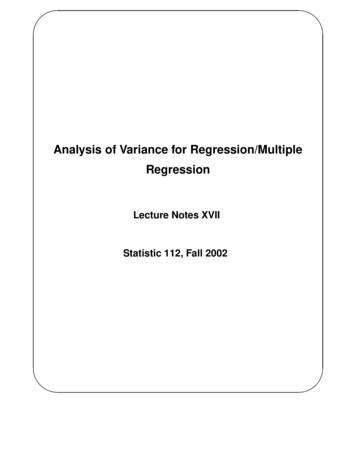
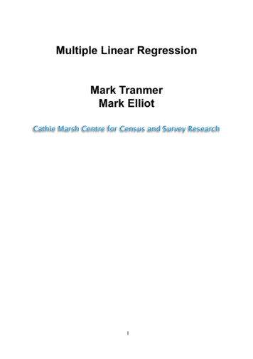
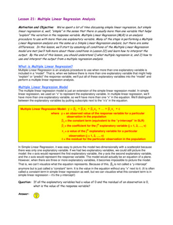
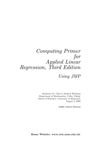
5The R squared is 97.1%, which did not drop significantly from the original model with all the 24predictors. Since the multiple coefficient of determination (R squared) is close to 1, it presents avery good fit. The Variance Inflation Factors (VIF) values looked reasonable since they are allunder 10, this means there is no multicollinearity between the 11 predictors. In addition, wetested the assumption of multiple regression for the selected equation above. The first test ofnormal distribution for the error, showed by Figure 1 and Figure 2, indicates the equation aboveis in fact a normal distribution with minimal outliers. The second assumption is to test theindependence of the error. We used the Durbin-Watson (DW) Statistic to prove that there is noserial correlation, thus, to prove the independence of the error. Using Minitab we found the DWis equal to 2.00286, which is close to 2 proving that the null hypothesis (ρє,ε-1 0) is reasonable.Therefore, the two assumptions were met.Using the given Analysis of Variance (ANOVA) Table by Minitab, we used the F test toevaluate the best regression equation for weight from those 11 selected variables. Thehypothesis test is:H0:β1 β2 β3 β4 β5 β6 β7 β8 β9 β10 β11 0H1: At least one of the β is not equal to zero.The F value is determined by the mean squared of regression divided by the mean squared oferror. Since the computed value of F 1518.51 is greater than 1.8, we reject the null hypothesisand conclude that the regression is significant at a significance level of 5%.Furthermore, we tested the Graphical Analysis of Residuals (residuals against fittedvalues) shown by Figure 3. We found that residual model against the fitted values is constant,with one influential point. This indicates the model is reasonable. Given the unusual observation
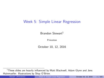
6output there were only 6 observations within the entire model where the X value gives it largeleverage.Moreover, we computed a similar regression analysis for the second model, leaving outthe shoulder girth instead of the chest girth, and found very similar results. The differencebetween the two predictive models for weight is that the VIF of the chest girth was close to 10,however the R squared is 0.1% higher. The two assumption hypotheses (shown by Figure 4 andFigure 5) are met as well. The F test (Table 3) is also significant. The model of residuals againstthe fitted values (Figure 6) is reasonable. In this analysis, we found only 4 unusual observationswhose X variable gives it large leverage.Section 3: Conclusion and recommendationFrom our analysis utilizing multiple methods of data processing technique, we havedetermined that two acceptable models are applicable to the data. We simplified the original 12body girths and 9 skeletal diameters factors to 8 dimensions, plus their weight, height, age andgender. The first model includes factors including prelvicbreadth, chestdepth, kneediam,chestgirth, waistgirth, hipgirth, forearmgirth, kneegirth, age, height, and dummy variable gender.The second model includes factors including prelvicbreadth, kneediam, shouldergirth, chestgirth,waistgirth, hipgirth, forearmgirth, kneegirth, age, height, and dummy variable gender. Sincethere exists multicollinearity between chestgirth and shouldergirth, we have to pick one of themin the prediction model.Applying regression analysis, best subsets, stepwise, Durbin-Watson (DW) statistic andPearson correlation test, we obtained the optimal linear regression prediction functions. For
7further analysis of the data, we recommend using multivariate multiple linear regression analysisthat includes response surface models.
8APPENDIXTable 1: Regression (weight vs. height)weight - 105 1.02 heightPredictorConstantheightCoef-105.0111.01762S 9.30804SE Coef7.5390.04399R-Sq 51.5%T-13.9323.13P0.0000.000VIF1.000R-Sq(adj) 51.4%Table 2: ANOVA (for the 1st best regression equation)SourceRegressionResidual 5.2F1518.51Table 3: ANOVA (for the 2nd best regression equation)SourceRegressionResidual 5.2F1538.01P0.000Figure 1: Assumption Test for the 1st best regression equationP0.000
9Figure2:Assumption Test for the 1st best regression equationFigure3: Graphical Analysis of Residuals for the 1st best regression equationFigure4:Assumption Test for the 2nd best regression equation
10Figure5:Assumption Test for the 1st best regression equationFigure3: Graphical Analysis of Residuals for the 2nd best regression equation
Applying regression analysis, best subsets, stepwise, Durbin-Watson (DW) statistic and Pearson correlation test, we obtained the optimal linear regression prediction functions. For . 7!! further analysis of the data, we recommend using multivariate multiple linear regression analysis