Transcription
Multiple Linear RegressionMark TranmerMark Elliot1
ContentsSection 1: Introduction.3Exam16.Exam11 . 4Predicted values. 5Residuals. 6Scatterplot of exam performance at 16 against exam performance at 11. 61.3 Theory for multiple linear regression.7Section 2: Worked Example using SPSS.10Section 3: Further topics . 36Stepwise. 46Section 4: BHPS assignment . 46Reading list. 47More theoretical:. 472
Section 1: Introduction1.1 OverviewA multiple linear regression analysis is carried out to predict the values of adependent variable, Y, given a set of p explanatory variables (x1,x2, .,xp). In thesenotes, the necessary theory for multiple linear regression is presented and examplesof regression analysis with census data are given to illustrate this theory. This courseon multiple linear regression analysis is therefore intended to give a practical outlineto the technique. Complicated or tedious algebra will be avoided where possible, andreferences will be given to more theoretical texts on this technique. Important issuesthat arise when carrying out a multiple linear regression analysis are discussed indetail including model building, the underlying assumptions, and interpretation ofresults. However, before we consider multiple linear regression analysis we beginwith a brief review of simple linear regression.1.2 Review of Simple linear regression.A simple linear regression is carried out to estimate the relationship between adependent variable, Y, and a single explanatory variable, x, given a set of data thatincludes observations for both of these variables for a particular population. Forexample, for a sample of n 17 pupils in a particular school, we might be interested inthe relationship of two variables as follows: Exam performance at age 16. The dependent variable, y (Exam16)Exam performance at age 11. The explanatory variable, x (Exam11)(n.b. we would ideally have a bigger sample, but this small sample illustrates theideas)3
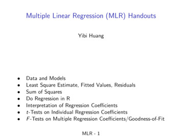
Exam16 565690407062455565667766We would carry out a simple linear regression analysis to predict the value of thedependent variable y, given the value of the explanatory variable, x. In this examplewe are trying to predict the value of exam performance at 16 given the examperformance at age 11.Before we write down any models we would begin such an analysis by plotting thedata as follows: Figure 1.1.We could then calculate a correlation coefficient to get a summary measure of thestrength of the relationship. For figure 1.1 we expect the correlation is highly positive(it is 0.87). If we want to fit a straight line to these points, we can perform a simplelinear regression analysis. We can write down a model of the following form.4
Where β0 the intercept and β1 is the slope of the line. We assume that the errorterms ei have a mean value of 0.The relationship between y and x is then estimated by carrying out a simple linearregression analysis. We will use the least squares criterion to estimate theequations, so that we minimise the sum of squares of the differences between theactual and predicted values for each observation in the sample. That is, we minimiseΣei2. Although there are other ways of estimating the parameters in the regressionmodel, the least squares criterion has several desirable statistical properties, mostnotably, that the estimates are maximum likelihood if the residuals ei are normallydistributed.For the example above, if we estimate the regression equation we get:where xi is the value of EXAM11 for the ith student.We could draw this line on the scatter plot. It is sometimes referred to as the line of yon x, because we are trying to predict y on the information provided by x.Predicted valuesThe first student in the sample has a value of 45 for EXAM16 and 55 for exam11.The predicted value of EXAM16 for this student is 47.661.5
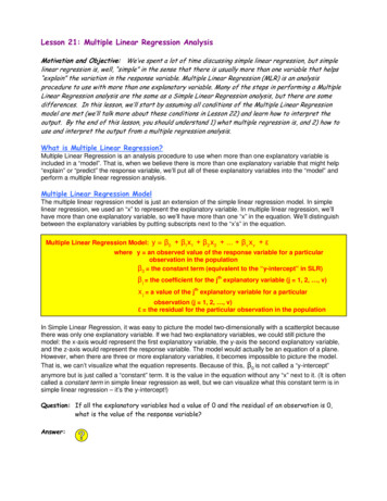
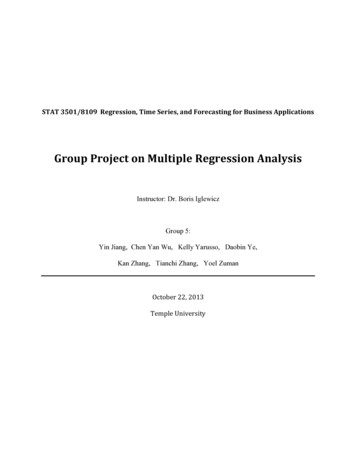
ResidualsWe know that the actual value of EXAM16 for the first student is 45, and thepredicted value is 47.661, therefore the residual may be calculated as the differencebetween the actual and predicted values of EXAM16. That is, 45 – 47.661 -2.661.Figure 1.2 Scatter plot, including the regression line.Scatterplot of exam performance at 16 against exam performance at 116
1.3 Theory for multiple linear regressionIn multiple linear regression, there are p explanatory variables, and the relationshipbetween the dependent variable and the explanatory variables is represented by thefollowing equation:Where:β0 is the constant term andβ1 to βp are the coefficients relating the p explanatory variables to the variables ofinterest.So, multiple linear regression can be thought of an extension of simple linearregression, where there are p explanatory variables, or simple linear regression canbe thought of as a special case of multiple linear regression, where p 1. The term‘linear’ is used because in multiple linear regression we assume that y is directlyrelated to a linear combination of the explanatory variables.Examples where multiple linear regression may be used include: Trying to predict an individual’s income given several socio-economiccharacteristics.Trying to predict the overall examination performance of pupils in ‘A’ levels, giventhe values of a set of exam scores at age 16.Trying to estimate systolic or diastolic blood pressure, given a variety of socioeconomic and behavioural characteristics (occupation, drinking smoking, ageetc).As is the case with simple linear regression and correlation, this analysis does notallow us to make causal inferences, but it does allow us to investigate how a set ofexplanatory variables is associated with a dependent variable of interest.In terms of a hypothesis test, for the case of a simple linear regression the nullhypothesis, H0 is that the coefficient relating the explanatory (x) variable to thedependent (y) variable is 0. In other words that there is no relationship between theexplanatory variable and the dependent variable. The alternative hypothesis H1 isthat the coefficient relating the x variable to the y variable is not equal to zero. Inother words there is some kind of relationship between x and y.7
In summary we would write the null and alternative hypotheses as:H0: β1 0H1: β1 08
A1: Aside: theory for correlation and simple linear regressionThe correlation coefficient, r, is calculated using:Where,Is the variance of x from the sample, which is of size n.Is the variance of y, and,Is the covariance of x and y.Notice that the correlation coefficient is a function of the variances of the twovariables of interest, and their covariance.In a simple linear regression analysis, we estimate the intercept, β0, and slope of theline, β1 as:9
Section 2: Worked Example using SPSSThis document shows how we can use multiple linear regression models with anexample where we investigate the nature of area level variations in the percentage of(self reported) limiting long term illness in 1006 wards in the North West of England.The data are from the 2001 UK Census.We will consider five variables here: The percentage of people in each ward who consider themselves to have alimiting long-term illness (LLTI)The percentage of people in each ward that are aged 60 and over (A60P)The percentage of people in each ward that are female (FEMALE)The percentage of people in each ward that are unemployed (of thoseEconomically active) (UNEM)The percentage of people in each ward that are ‘social renters’ (i.e .rent fromthe local authority). (SRENT).The dependent variable will be LLTI and we will investigate whether we can explainward level variations in LLTI with A60P, FEMALE, UNEM, SRENTWe will consider:1. Whether this model makes sense substantively2. Whether the usual assumptions of multiple linear regression analysis are metwith these data3. How much variation in LLTI the four explanatory variables explain4. Which explanatory variables are most ‘important’ in this model5. What is the nature of the relationship between LLTI and the explanatoryvariables.6. Are there any wards where there are higher (or lower) than expected levels ofLLTI given the explanatory variables we are considering here.But first we will do some exploratory data analysis (EDA). It is always a good idea toprecede a regression analysis with EDA. This may be univariate: descriptives,boxplots, histograms, bivariate: correlations, scatter plots, and occasionallymultivariate e.g. principal components analysis.10
Univariate EDA - descriptives11
12
Univariate EDA – boxplots13
Bivariate EDA - correlationsCorrelations14
15
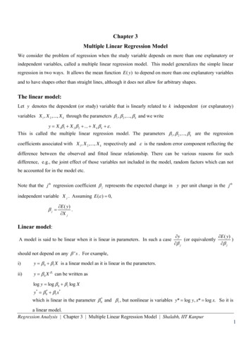
Bivariate EDA - Scatterplot16
Double click on the graph to go into the graph editor window 17
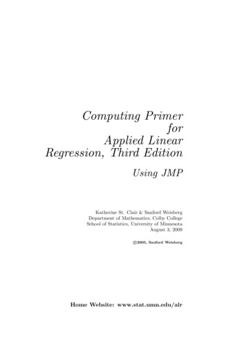
Choose – Elements, Fit line, Linear to fit a simple linear regression line of % LLTI on% social rented.18
19
The simple linear regression has an R squared value of 0.359. i.e. it explains 35.9%of the ward level variation in % LLTI20
Bivariate Analysis - Simple Linear RegressionLet us continue with the example where the dependent variable is % llti and there isa single explanatory variable, % social rented. Hence we begin with a simple linearregression analysis. We will then add more explanatory variables in a multiple linearregression analysis.To perform a linear regression analysis, go to theanalyze regression linearmenu options.Choose the dependent and independent (explanatory) variables you require. Thedefault ‘enter’ method puts all explanatory variables you specify in the model, in theorder that you specify them. Note that the order in unimportant in terms of themodeling process.There are other methods available for model building, based on statisticalsignificance, such as backward elimination or forward selection but when building themodel on a substantive basis, the enter method is best: variables are included in theregression equation regardless of whether or not they are statistically significant.21
22
Regressionthe table above confirms that the dependent variable is % llti and the explanatoryvariable here is % social rented.the table above shows that we have explained about 35.9% of the variation in % lltiwith the single explanatory variable, % social rented. In general quote the ‘adjusted rsquare’ figure. When the sample size, n, is large, r square and adjusted r square willusually be identical or very close. For small n, adjusted r square takes the sample23
size (and the number of explanatory variables in the regression equation) intoaccount.the ANOVA table above indicates that the model, as a whole, is a significant fit to thedata.The coefficients table above shows that: the constant, or intercept term for the line of best fit, when x 0, is 17.261(%).The slope, or coefficient for % social rented, is positive: areas with moresocial renting tend to be associated with areas with more limiting long termillness.The slope coefficient is 0.178 with a standard error of .008.The t value slope coefficient / standard error 23.733This is highly statistically significant (p 0.05) the usual 5% significancelevelThe standardized regression coefficient provides a useful way of seeing whatthe impact of changing the explanatory variable by one standard deviation.The standardized coefficient is 0.599 – a one standard deviation change inthe explanatory variable results in a 0.599 standard deviation change in thedependent variable % llti.the theoretical model isor24
whereis the intercept (constant) term andis the slope term; the coefficient that relates the value of SOCIAL P to theexpected value of LLTI.From the results above, our estimated equation is:25
Multiple linear regression analysisWe will now add some more explanatory variables so that we now have a multiplelinear regression mode, which now contains:Social rented, Age, female and age 60 plus as explanatory variables.26
RegressionThis multiple linear regression model, with four explanatory variables, now has an Rsquared value of 0.675. 67.5 % of the variation in % LLTI can be explained by thismodel.Once again, the model, as a whole, is a significant fit to the data.27
From the table above we see that: All the explanatory variables are statistically significant.All have positive coefficients – for each explanatory variable a greaterpercentage is associated with a higher level of LLTITaking % aged 60 and over as an example, we see that having controlled forunemp, female and social rented (i.e. holding these variables constant), forevery 1% increase in the % of 60 and over, there is an increase of 0.33% inthe predicted value of LLTI.The theoretical model here is:The estimated model here is:28
We notice that the variables % unemployed (of all economically active) and % socialrented are very highly correlated. We can assess the impact of the correlation on theregression results by leaving one of the variables, % unemployed, out of the multiplelinear regression analysis.RegressionWith 3 predictors ( a constant), we see that we can explain 51.7 % of the variationin % LLTI.29
The estimated model here is:Assumption checking.We can check many of the assumptions of the multiple linear regression analysis byproducing plots. Based on the results of the last model (with 3 explanatory variables)we can produce plots by clicking the ‘plots’ button, which appears in the windowwhen we specify the model in analyze regression linear. Click ‘histogram’ and‘normal probability plot’ to obtain the full range of plots:30
31
32
33
Also in the menu where we specify the regression equation via analyze regression linear is a ‘save’ button, where we can tick values, residuals and measures to beadded, as new variables, to the worksheet (i.e. the dataset) we are using. Here wehave saved the unstandardised and standardised residuals and predicted values:34
new variables are added to the worksheet calledpre 1 unstandardised predictedres 1 unstandardised residualzpr 1 standardised predictedzre 1 standardised residualthe suffix 1 in the variable names indicates these are the first set of residuals wehave saved. If we re-specified the model and saved the residuals, these variablenames would have the suffix 2 etc A large (positive) standardized residual i.e. 2 from the model indicates an areawhere, even when accounting for the explanatory variables in the model, there is stilla higher-than-expected level of LLTI in that ward. Conversely a standardized residual -2 indicated an area that, even when accounting for the explanatory variables,there is still a lower than expected level of LLTI.35
Section 3: Further topics3.1 Checking the assumptionsMost of the underlying assumptions of multiple linear regression can be assessed byexamining the residuals, having fitted a model. The various assumptions are listedbelow. Later, we will see how we can assess whether these assumptions hold byproducing the appropriate plots.The main assumptions are:1. That the residuals have constant variance, whatever the value of the dependentvariable. This is the assumption of homoscedasticity. Sometimes textbooksrefer to heteroscedasticity. This is simply the opposite of homoscedasticity.2. That there are no very extreme values in the data. That is, that there are nooutliers.3. That the residuals are normally distributed.4. That the residuals are not related to the explanatory variables.5. We also assume that the residuals are not correlated with one another.Residual plots.1. By plotting the predicted values against the residuals, we can assess thehomoscedasticity assumption. Often, rather than plotting the unstandardised orraw values, we would plot the standardised predicted values against thestandardised residuals. (Note that a slightly different version of the standardisedresidual is called the studentized residual, which are residuals standardised by theirown standard errors. See Plewis page 15 ff for further discussion of these).36
Examples from 1991 census dataset for districts in the North WestWe can also assess the assumption that there are no outliers in our data from theabove plot. If there was an extreme value in the standardised predicted values orstandardised residuals (say greater/less than /- 3), we should look at the sampleunit (in this case the district) that corresponds to the residual. We should considerthe following: is the data atypical of the general pattern for this sample unit? Has theinformation been recorded/entered into the computer properly for this sample unit? Isthere a substantive reason why this outlier occurs: have we left an importantexplanatory variable out of the regression analysis? In many cases an outlier willaffect the general estimate of the regression line, because the least squaresapproach will try to minimise the distance between the outlier and the regressionline. In some cases the extreme point will move the line away from the generalpattern of the data. That is, the outlier will have leverage on the regression line. Inmany cases we would consider deleting an outlier from the sample, so that we get abetter estimate of the relationship for the general pattern on the data. The above plotsuggests that, for our data, there are no outliers.We can assess the assumption that the residuals are normally distributed byproducing a normal probability plot (sometimes called a quantile-quantile or q-q plot).37
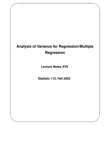
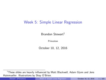
For this plot, the ordered values of the standardised residuals are plotted against theexpected values from the standard normal distribution. If the residuals are normallydistributed, they should lie, approximately, on the diagonal. The figure below showsthe normal probability plot for our example.The fourth assumption listed above is that the residuals are not related in some wayto the explanatory variables. We could assess this by plotting the standardisedresidual against the values of each explanatory variable. If a relationship does seemto exist on this plot, we need to consider putting extra terms in the regressionequation. For example, there may be a quadratic relationship between the residualand explanatory variable, as indicated by a ‘U’ or ‘n’ shaped curve of the points. Inorder to take into account this quadratic relationship, we would consider adding thesquare of the explanatory variable to the variables included in the model, so that themodel includes a quadratic (x2) term. E.g. if there appeared to be a quadraticrelationship between the residuals and age, we could add age2 to the model.38
The above plot shows a plot of an explanatory variables – AGE60P – against thestandardised residual. If the plot had an obvious pattern it would be sensible toconsider including further explanatory variables in the model. There does not seemto be an obvious pattern here, but with only 43 observations, it is not easy to tellwhether or not a pattern exists.In general it should be borne in mind that you should have a reasonable size sampleto carry out a multiple linear regression analysis when you have a lot of explanatoryvariables.There is no simple answer as to how many observations you need, but in general thebigger the sample, the better.3.2 Multicollinearity.By carrying out a correlation analysis before we fit the regression equations, we cansee which, if any, of the explanatory variables are very highly correlated and avoidthis problem (or at least this will indicate why estimates of regression coefficientsmay give values very different from those we might expect). For pairs of explanatoryvariables with have very high correlations 0.8 or very low correlations 0.8 wecould consider dropping one of the explanatory variables from the model.39
3.3 Transformations:In some situations the distribution of the dependent variable is not normal, butinstead is positively or negatively skewed. For example the distribution of income,and similar variables such as hourly pay, tends to be positively skewed because afew people earn a very high salary. Below is an example of the distribution of hourlypay. As can be seen, it is positively skewed.If we now take the natural log (LN) of the hourly wage we can see that the resultingdistribution is much more ‘normal’.40
Later we will do some multiple linear regression modelling using log(hourly wage) asthe dependent variable.3.4 Dummy variablesSuppose we were interested in investigating differences, with respect to the yvariable (e.g. log(income), in three different ethnic groups. Hence we would have anethnic group variable with three categories: Afro Caribbean, Pakistani, Indian. Wewould need to create dummy variables to include this categorical variable in themodelFor example we could use this dummy variable scheme, where ‘afro-caribbean’ isthe reference ere D1 is the dummy variable to represent the Pakistani ethnic group andD2 is the dummy variable to represent the Indian ethnic group41
Hence the estimate of the coefficient β0 gives the average log(income) for the AfroCaribbean ethnic group. The estimate of β1 shows how log(income) differs onaverage for Indian vs Afro-Caribbean ethnic group and the estimate of coefficient β2shows how log income differs on average for Pakistani vs Afro Caribbean ethnicgroup. If we are interested in the way in which log income differs on average for theIndian vs Pakistani ethnic group we can find this out by subtracting the estimate of β2from the estimate of β1.Dummy variables can be created in SPSS via compute variable or via recode. Boththese options appear in the transform menu in SPSS.3.5 Interactions:Interactions enable us to assess whether the relationship between the dependentvariable and one explanatory variable might change with respect to values of anotherexplanatory variable.For example, consider a situation where we have a sample of pupils, and thedependent variable is examination performance at 16 (exam16) which we are tryingto predict with a previous measure of examination performance based on an examthe pupils took when they were 11 years old (exam11). Suppose we have anotherexplanatory variable, gender.There are three usual things that might be the case for this example (assuming thatthere is some kind of a relationship between exam16 and exam11).(a) The relationship between exam16 and exam 11 is identical for boys and girls.(b) The relationship between exam16 and exam11 has a different intercept(overall average) for boys than girls but the nature of the relationship (i.e. theslope) is the same for boys and for girls). In graph (b) below the top line mightrefer to girls and the bottom line to boys.(c) The relationship between exam16 and exam11 has a different intercept and adifferent slope for boys and girls4. In graph (c) below the line with the lowerintercept but steeper slope might refer to boys and the line with the higherintercept and shallower slope to girls.And one other possibility that is less likely to occur in general.(d) A fourth possibility is that the slope is different for girls and boys but theintercept is identical. In this graph (d, below) one of the lines would refer togirls and the other to boys.42
Graphical representations of all four possibilities are shown below:(a)(b)(c)43
The simplest model, represented schematically by graph (a) above is one whereexam16 and exam11 are positively associated, but there is no difference in thisrelationship for girls compared with boys. In other words, a single line applies to bothgenders. The equation for this line is:(a)where exam16 and exam11 are continuous exam scoresIf we now consider graph b we might find that there is an overall difference in thelevel of exam average exam scores but once we have accounted for this overalldifference, the relationship between exam16 and exam11 is the same for girls andboys. That is, the lines have the same slope and are therefore parallel.We can represent this situation via a main effects model where we now have asecond explanatory variable. This time it is a categorical (dummy) variable, wheregender 0 for boys and gender 1 for girls. Equation (b) is hence a main effectsmodel relating exam11 and gender to exam11.(b)Interactions can also be added to the model (this would be appropriate if case (c)applies).(c)To create an interaction term such as exam11.gender we simply multiply the twovariables exam11 and gender together to create a new variable e.g. ex11gen wethen add this to the model as a new explanatory variable. In general you shouldalways leave each of the single variables that make up the interaction term in themodel when the interaction term is added.3.6 Quadratic Relationships.Sometimes a linear relationship between dependent and explanatory variable maynot be appropriate and this is often evident when a scatter plot is produced. Forexample the linear relationship and quadratic (i.e. curved) relationship for log(hourlywage) vs age are shown below. It seems that although age as a single measuredoes not explain all the variation in log(hourly wage) it is apparent that therelationship between log(hourly wage) and age is better summarised with a quadraticcurve than a straight line.44
figure (a) abovefigure (b) aboveIt is easy to estimate a curve as shown above using SPSS. We first create a newvariable: agesq age2. We then simply add agesqu into the regression equation asa new explanatory variable.Hence the equation the straight line shown in figure (a) is:45
And the equation for the curve shown in figure (b) is:Which we could also write equivalently as:3.6 Model selection methodsIn some cases, especially when there are a large number of explanatory variables,we might use statistical criteria to include/exclude explanatory variables, especially ifwe are interested in the ‘best’ equation to predict the dependent variable. This is adifferent fundamental approach to the substantive approach where variables areincluded on the basis of the research question and this variables are often chosengiven the results previous research on the topic and are also influenced by ‘commonsense’ and data availability.Two examples of selection methods are backward elimination, and stepwise. Themain disadvantage of these methods is that we might miss out important theoreticalvariables, or interactions. Two selection methods are briefly described below. SeeHowell page 513 ff for a more detailed description of the methods.Backward elimination.Begin with a model that includes all the explanatory variables. Remove the one thatis least significant. Refit the model, having removed the least significant explanatoryvariable, remove the least significant explanatory variable from the remaining set,refit the model, and so on, until some ‘stopping’ criterion is met: usually that all theexplanatory variables that are included in the model are significant.StepwiseMore or less the reverse of backward elimination, in that we start with no explanatoryvariables in the model, and then build the model up, step-by-step. We begin byincluding the variable most highly correlated to the dependent variable in the model.Then include the next most correlated variable, allowing for the first explanatoryvariable in the model, and keep adding explanatory variables until no furthervariables are significant. In this approach, it is possible to delete a variable that hasbeen included at an earlier step but is no longer significant, given the explanatoryvariables that were added later. If we ignore this possibility, and do not allow anyvariables that have already been added to the model to be deleted, this modelbuilding procedure is called forward selection.Section 4: BHPS assignmentUsing the dataset bhps.sav produce a short report of a multiple regression analysisof the log (hourly wage). The dataset is on the blackboard site.46
The report should be between 500-1000 words and might include:Appropriate exploratory analysis.Appropriate tests of assumptions.Dummy variables.Interaction terms.Squared terms.Multiple models (i.e. evidence of a model selection process).Don’t worry about presentational issues for this assignment; we are not afterpolished pieces of work at this stage. You can cut and paste any relevant SPSSoutput into appendices. The important point is to the interpretation of the output; thereader should be able to understand the analytical process you have been through.So explain your recodes, dummy variables model selection choices etc.Reading listBryman A and Cramer D (1
A multiple linear regression analysis is carried out to predict the values of a dependent variable, Y, given a set of p explanatory variables (x1,x2, .,xp). In these notes, the necessary theory for multiple linear regression is presented and examples of regression analysis with census data are given to illustrate this theory.