Transcription
Week 5: Simple Linear RegressionBrandon Stewart1PrincetonOctober 10, 12, 20161These slides are heavily influenced by Matt Blackwell, Adam Glynn and JensHainmueller. Illustrations by Shay O’Brien.Stewart (Princeton)Week 5: Simple Linear RegressionOctober 10, 12, 20161 / 103
Where We’ve Been and Where We’re Going.Last WeekIIhypothesis testingwhat is regressionThis WeekIMonday:FFImechanics of OLSproperties of OLSWednesday:FFFhypothesis tests for regressionconfidence intervals for regressiongoodness of fitNext WeekIImechanics with two regressorsomitted variables, multicollinearityLong RunIprobability inference regressionQuestions?Stewart (Princeton)Week 5: Simple Linear RegressionOctober 10, 12, 20162 / 103
MacrostructureThe next few weeks,Linear Regression with Two RegressorsMultiple Linear RegressionBreak WeekRegression in the Social ScienceWhat Can Go Wrong and How to Fix It Week 1What Can Go Wrong and How to Fix It Week 2 / ThanksgivingCausality with Measured ConfoundingUnmeasured Confounding and Instrumental VariablesRepeated Observations and Panel DataA brief comment on exams, midterm week etc.Stewart (Princeton)Week 5: Simple Linear RegressionOctober 10, 12, 20163 / 103
1Mechanics of OLS2Properties of the OLS estimator3Example and Review4Properties Continued5Hypothesis tests for regression6Confidence intervals for regression7Goodness of fit8Wrap Up of Univariate Regression9Fun with Non-LinearitiesStewart (Princeton)Week 5: Simple Linear RegressionOctober 10, 12, 20164 / 103
The population linear regression functionThe (population) simple linear regression model can be stated as thefollowing:r (x) E [Y X x] β0 β1 xThis (partially) describes the data generating process in thepopulationY dependent variableX independent variableβ0 , β1 population intercept and population slope (what we want toestimate)Stewart (Princeton)Week 5: Simple Linear RegressionOctober 10, 12, 20165 / 103
The sample linear regression functionThe estimated or sample regression function is:rb(Xi ) Ybi βb0 βb1 Xiβb0 , βb1 are the estimated intercept and slopeYbi is the fitted/predicted valueWe also have the residuals, ubi which are the differences between thetrue values of Y and the predicted value:ubi Yi YbiYou can think of the residuals as the prediction errors of ourestimates.Stewart (Princeton)Week 5: Simple Linear RegressionOctober 10, 12, 20166 / 103
Overall Goals for the WeekLearn how to run and read regressionMechanics: how to estimate the intercept and slope?Properties: when are these good estimates?Uncertainty: how will the OLS estimator behave in repeated samples?Testing: can we assess the plausibility of no relationship (β1 0)?Interpretation: how do we interpret our estimates?Stewart (Princeton)Week 5: Simple Linear RegressionOctober 10, 12, 20167 / 103
What is OLS?An estimator for the slope and the intercept of the regression lineWe talked last week about ways to derive this estimator and wesettled on deriving it by minimizing the squared prediction errors ofthe regression, or in other words, minimizing the sum of the squaredresiduals:Ordinary Least Squares (OLS):(βb0 , βb1 ) arg minb0 ,b1nX(Yi b0 b1 Xi )2i 1In words, the OLS estimates are the intercept and slope that minimizethe sum of the squared residuals.Stewart (Princeton)Week 5: Simple Linear RegressionOctober 10, 12, 20168 / 103
Graphical ExampleHow do we fit the regression line Ŷ β̂0 β̂1 X to the data? 0 1Stewart (Princeton)Week 5: Simple Linear RegressionOctober 10, 12, 20169 / 103
Graphical ExampleHow do we fit the regression line Ŷ β̂0 β̂1 X to the data?Answer: We will minimize the squared sum of residualsResidual ui is “part”of Yi not predicted ui Yi Y in 2 umin 0, 1Stewart (Princeton)i 1iWeek 5: Simple Linear RegressionOctober 10, 12, 20169 / 103
Deriving the OLS estimatorLet’s think about n pairs of sample observations:(Y1 , X1 ), (Y2 , X2 ), . . . , (Yn , Xn )Let {b0 , b1 } be possible values for {β0 , β1 }Define the least squares objective function:S(b0 , b1 ) nX(Yi b0 b1 Xi )2 .i 1How do we derive the LS estimators for β0 and β1 ? We want tominimize this function, which is actually a very well-defined calculusproblem.123Take partial derivatives of S with respect to b0 and b1 .Set each of the partial derivatives to 0Solve for {b0 , b1 } and replace them with the solutionsTo the board we go!Stewart (Princeton)Week 5: Simple Linear RegressionOctober 10, 12, 201610 / 103
The OLS estimatorNow we’re done! Here are the OLS estimators:βb0 Y βb1 XPn(Xi X )(Yi Y )bβ1 i 1Pn2i 1 (Xi X )Stewart (Princeton)Week 5: Simple Linear RegressionOctober 10, 12, 201611 / 103
Intuition of the OLS estimatorThe intercept equation tells us that the regression line goes throughthe point (Y , X ):Y βb0 βb1 XThe slope for the regression line can be written as the following:Pnβb1 i 1 (Xi X )(Yi Pn2i 1 (Xi X )Y) Sample Covariance between X and YSample Variance of XThe higher the covariance between X and Y , the higher the slope willbe.Negative covariances negative slopes;positive covariances positive slopesWhat happens when Xi doesn’t vary?What happens when Yi doesn’t vary?Stewart (Princeton)Week 5: Simple Linear RegressionOctober 10, 12, 201612 / 103
A Visual Intuition for the OLS EstimatorStewart (Princeton)Week 5: Simple Linear RegressionOctober 10, 12, 201613 / 103
A Visual Intuition for the OLS EstimatorStewart (Princeton)Week 5: Simple Linear RegressionOctober 10, 12, 201613 / 103
A Visual Intuition for the OLS Estimator Stewart (Princeton) Week 5: Simple Linear Regression - October 10, 12, 201613 / 103
Mechanical properties of OLSLater we’ll see that under certain assumptions, OLS will have nicestatistical properties.But some properties are mechanical since they can be derived fromthe first order conditions of OLS.1The residuals will be 0 on average:n1Xubi 0ni 12The residuals will be uncorrelated with the predictorc is the sample covariance):(covc i , ubi ) 0cov(X3The residuals will be uncorrelated with the fitted values:c Ybi , ubi ) 0cov(Stewart (Princeton)Week 5: Simple Linear RegressionOctober 10, 12, 201614 / 103
OLS slope as a weighted sum of the outcomesOne useful derivation is to write the OLS estimator for the slope as aweighted sum of the outcomes.βb1 nXWi Yii 1Where here we have the weights, Wi as:(Xi X )Wi Pn2i 1 (Xi X )This is important for two reasons. First, it’ll make derivations latermuch easier. And second, it shows that is just the sum of a randomvariable. Therefore it is also a random variable.To the board!Stewart (Princeton)Week 5: Simple Linear RegressionOctober 10, 12, 201615 / 103
1Mechanics of OLS2Properties of the OLS estimator3Example and Review4Properties Continued5Hypothesis tests for regression6Confidence intervals for regression7Goodness of fit8Wrap Up of Univariate Regression9Fun with Non-LinearitiesStewart (Princeton)Week 5: Simple Linear RegressionOctober 10, 12, 201616 / 103
Sampling distribution of the OLS estimatorRemember: OLS is an estimator—it’s a machine that we plug datainto and we get out estimates.Sample 1: {(Y1 , X1 ), . . . , (Yn , Xn )}(βb0 , βb1 )1Sample 2: {(Y1 , X1 ), . . . , (Yn , Xn )}(βb0 , βb1 )2.OLSSample k 1: {(Y1 , X1 ), . . . , (Yn , Xn )}Sample k: {(Y1 , X1 ), . . . , (Yn , Xn )}.(βb0 , βb1 )k 1(βb0 , βb1 )kJust like the sample mean, sample difference in means, or the samplevarianceIt has a sampling distribution, with a sampling variance/standarderror, etc.Let’s take a simulation approach to demonstrate:IIPretend that the AJR data represents the population of interestSee how the line varies from sample to sampleStewart (Princeton)Week 5: Simple Linear RegressionOctober 10, 12, 201617 / 103
Simulation procedure123Draw a random sample of size n 30 with replacement usingsample()Use lm() to calculate the OLS estimates of the slope and interceptPlot the estimated regression lineStewart (Princeton)Week 5: Simple Linear RegressionOctober 10, 12, 201618 / 103
11109876Log GDP per capita growth12Population Regression12345678Log Settler MortalityStewart (Princeton)Week 5: Simple Linear RegressionOctober 10, 12, 201619 / 103
11109876Log GDP per capita growth12Randomly sample from AJR12345678Log Settler MortalityStewart (Princeton)Week 5: Simple Linear RegressionOctober 10, 12, 201620 / 103
Sampling distribution of OLSYou can see that the estimated slopes and intercepts vary from sampleto sample, but that the “average” of the lines looks about right.100300Sampling distribution of slopesFrequency30000100FrequencySampling distribution of intercepts68101214-1.5 β0-1.0-0.50.00.5 β1Is this unique?Stewart (Princeton)Week 5: Simple Linear RegressionOctober 10, 12, 201621 / 103
Assumptions for unbiasedness of the sample meanWhat assumptions did we make to prove that the sample mean wasunbiased?E[X ] µJust one: random sampleWe’ll need more than this for the regression caseStewart (Princeton)Week 5: Simple Linear RegressionOctober 10, 12, 201622 / 103
Our goalWhat is the sampling distribution of the OLS slope?βb1 ?(?, ?)We need fill in those ?s.We’ll start with the mean of the sampling distribution. Is theestimator centered at the true value, β1 ?Most of our derivations will be in terms of the slope but they apply tothe intercept as well.Stewart (Princeton)Week 5: Simple Linear RegressionOctober 10, 12, 201623 / 103
OLS Assumptions Preview1Linearity in Parameters: The population model is linear in itsparameters and correctly specified2Random Sampling: The observed data represent a random samplefrom the population described by the model.3Variation in X : There is variation in the explanatory variable.4Zero conditional mean: Expected value of the error term is zeroconditional on all values of the explanatory variable5Homoskedasticity: The error term has the same variance conditionalon all values of the explanatory variable.6Normality: The error term is independent of the explanatory variablesand normally distributed.Stewart (Princeton)Week 5: Simple Linear RegressionOctober 10, 12, 201624 / 103
Hierarchy of OLS Assumptions!"# %&'(%) * (,(* #-'./0%) *1(./(%) */ *2*3 4/(-#" #--*5) -/-,# '6*@(A--B?(.C)D*EF 3GH*I-680,)%'*! J#.# '#*************EK*( "*!LH"5:(--/'(:* ?*EF3GH*98(::B9(80:#*! J#.# '#***E,*( "*NH*1(./(%) */ *2*1(./(%) */ *2*1(./(%) */ *2*7( ")8*9(80:/ ;*7( ")8*9(80:/ ;*7( ")8*9(80:/ ;* / #(./,6*/ * (.(8#,#.-* / #(./,6*/ * (.(8#,#.-* / #(./,6*/ * (.(8#,#.-* #.)*5) "/%) (:*?#( * #.)*5) "/%) (:*?#( * #.)*5) "/%) (:*?#( -*Stewart (Princeton)Week 5: Simple Linear RegressionOctober 10, 12, 201625 / 103
OLS Assumption IAssumption (I. Linearity in Parameters)The population regression model is linear in its parameters and correctlyspecified as:Y β0 β1 X1 uNote that it can be nonlinear in variablesIIOK: Y β0 β1 X u orY β0 β1 X 2 u orY β0 β1 log (X ) uNot OK: Y β0 β12 X u orY β0 exp(β1 )X uβ0 , β1 : Population parameters — fixed and unknownu: Unobserved random variable with E [u] 0 — captures all otherfactors influencing Y other than XWe assume this to be the structural model, i.e., the model describingthe true process generating YStewart (Princeton)Week 5: Simple Linear RegressionOctober 10, 12, 201626 / 103
OLS Assumption IIAssumption (II. Random Sampling)The observed data:(yi , xi ) for i 1, ., nrepresent an i.i.d. random sample of size n following the population model.Data examples consistent with this assumption:A cross-sectional survey where the units are sampled randomlyPotential Violations:Time series data (regressor values may exhibit persistence)Sample selection problems (sample not representative of thepopulation)Stewart (Princeton)Week 5: Simple Linear RegressionOctober 10, 12, 201627 / 103
OLS Assumption IIIAssumption (III. Variation in X ; a.k.a. No Perfect Collinearity)The observed data:xi for i 1, ., nare not all the same value.Satisfied as long as there is some variation in the regressor X in thesample.Why do we need this?Pnβ̂1 (x x̄)(yi i 1Pn i2i 1 (xi x̄)ȳ )This assumption is needed just to calculate β̂, i.e. identifying β̂.In fact, this is the only assumption needed for using OLS as a pure datasummary.Stewart (Princeton)Week 5: Simple Linear RegressionOctober 10, 12, 201628 / 103
Stuck in a moment-2-1Y01Why does this matter? How would you draw the line of best fitthrough this scatterplot, which is a violation of this assumption?-3-2-10123XStewart (Princeton)Week 5: Simple Linear RegressionOctober 10, 12, 201629 / 103
OLS Assumption IVAssumption (IV. Zero Conditional Mean)The expected value of the error term is zero conditional on any value of theexplanatory variable:E [u X ] 0E [u X ] 0 implies a slightly weaker condition Cov(X , u) 0Given random sampling, E [u X ] 0 also implies E [ui xi ] 0 for all iViolations:Recall that u represents all unobserved factors that influence YIf such unobserved factors are also correlated with X , Cov(X , u) 6 0Example: Wage β0 β1 education u. What is likely to be in u? It must be assumed E [ability educ low ] E [ability educ high]Stewart (Princeton)Week 5: Simple Linear RegressionOctober 10, 12, 201630 / 103
Violating the zero conditional mean assumptionHow does this assumption get violated? Let’s generate data from thefollowing model:Yi 1 0.5Xi uiBut let’s compare two situations:12Where the mean of ui depends on Xi (they are correlated)No relationship between them (satisfies the assumption)Stewart (Princeton)Week 5: Simple Linear RegressionOctober 10, 12, 201631 / 103
Violating the zero conditional mean assumption432-2-101Y-2-101Y2345Assumption 4 not violated5Assumption 4 violated-3-2-10123-3XStewart (Princeton)-2-10123XWeek 5: Simple Linear RegressionOctober 10, 12, 201632 / 103
Unbiasedness (to the blackboard)With Assumptions 1-4, we can show that the OLS estimator for the slopeis unbiased, that is E [βb1 ] β1 .Stewart (Princeton)Week 5: Simple Linear RegressionOctober 10, 12, 201633 / 103
Unbiasedness of OLSTheorem (Unbiasedness of OLS)Given OLS Assumptions I–IV:E [β̂0 ] β0andE [β̂1 ] β1The sampling distributions of the estimators β̂1 and β̂0 are centered aboutthe true population parameter values β1 and β0 .Stewart (Princeton)Week 5: Simple Linear RegressionOctober 10, 12, 201634 / 103
Where are we?Now we know that, under Assumptions 1-4, we know thatβb1 ?(β1 , ?)That is we know that the sampling distribution is centered on thetrue population slope, but we don’t know the population variance.Stewart (Princeton)Week 5: Simple Linear RegressionOctober 10, 12, 201635 / 103
Sampling variance of estimated slopeIn order to derive the sampling variance of the OLS estimator,12345LinearityRandom (iid) sampleVariation in XiZero conditional mean of the errorsHomoskedasticityStewart (Princeton)Week 5: Simple Linear RegressionOctober 10, 12, 201636 / 103
Variance of OLS EstimatorsHow can we derive Var[β̂0 ] and Var[β̂1 ]? Let’s make the following additionalassumption:Assumption (V. Homoskedasticity)The conditional variance of the error term is constant and does not vary as afunction of the explanatory variable:Var[u X ] σu2This implies Var[u] σu2 all errors have an identical error variance (σu2i σu2 for all i)Taken together, Assumptions I–V imply:E [Y X ] β0 β1 XVar[Y X ] σu2Violation: Var[u X x1 ] 6 Var[u X x2 ] called heteroskedasticity.Assumptions I–V are collectively known as the Gauss-Markov assumptionsStewart (Princeton)Week 5: Simple Linear RegressionOctober 10, 12, 201637 / 103
Deriving the sampling variancevar[βb1 X1 , . . . , Xn ] ?Stewart (Princeton)Week 5: Simple Linear RegressionOctober 10, 12, 201638 / 103
Variance of OLS EstimatorsTheorem (Variance of OLS Estimators)Given OLS Assumptions I–V (Gauss-Markov Assumptions):σu2σu2 2SSTxi 1 (xi x̄) 1x̄ 22Var[β̂0 X ] σu Pn2ni 1 (xi x̄)Var[β̂1 X ] Pnwhere Var[u X ] σu2 (the error variance).Stewart (Princeton)Week 5: Simple Linear RegressionOctober 10, 12, 201639 / 103
Understanding the sampling varianceσu22i 1 (Xi X )var[βb1 X1 , . . . , Xn ] PnWhat drives the sampling variability of the OLS estimator?IIIThe higher the variance of Yi , the higher the sampling varianceThe lower the variance of Xi , the higher the sampling varianceAs we increase n, the denominator gets large, while the numerator isfixed and so the sampling variance shrinks to 0.Stewart (Princeton)Week 5: Simple Linear RegressionOctober 10, 12, 201640 / 103
Estimating the Variance of OLS EstimatorsHow can we estimate the unobserved error variance Var [u] σu2 ?We can derive an estimator based on the residuals:ûi yi ŷi yi β̂0 β̂1 xiRecall: The errors ui are NOT the same as the residuals ûi .Intuitively, the scatter of the residuals around the fitted regression line shouldreflect the unseen scatter about the true population regression line.We can measure scatter with the mean squared deviation:MSD(û) nnX1X 2 1(ûi û)ûi2nni 1i 1Intuitively, which line is likely to be closer to the observed sample values on Xand Y , the true line yi β0 β1 xi or the fitted regression line ŷi β̂0 β̂1 xi ?Stewart (Princeton)Week 5: Simple Linear RegressionOctober 10, 12, 201641 / 103
Estimating the Variance of OLS EstimatorsBy construction, the regression line is closer since it is drawn to fit theactual sample we haveSpecifically, the regression line is drawn so as to minimize the sum of thesquares of the distances between it and the observationsSo the spread of the residuals MSD(û) will slightly underestimate the errorvariance Var[u] σu2 on averageIn fact, we can show that with a single regressor X we have:E [MSD(û)] n 2 2σu (degrees of freedom adjustment)nThus, an unbiased estimator for the error variance is:σ̂u2 nnnn 1X1 X 2MSD(û) ûi ûin 2n 2nn 2i 1i 1We plug this estimate into the variance estimators for β̂0 and β̂1 .Stewart (Princeton)Week 5: Simple Linear RegressionOctober 10, 12, 201642 / 103
Where are we?Under Assumptions 1-5, we know that σu2bβ1 ? β1 , Pn2i 1 (Xi X )Now we know the mean and sampling variance of the samplingdistribution.Next Time: how does this compare to other estimators for thepopulation slope?Stewart (Princeton)Week 5: Simple Linear RegressionOctober 10, 12, 201643 / 103
Where We’ve Been and Where We’re Going.Last WeekIIhypothesis testingwhat is regressionThis WeekIMonday:FFImechanics of OLSproperties of OLSWednesday:FFFhypothesis tests for regressionconfidence intervals for regressiongoodness of fitNext WeekIImechanics with two regressorsomitted variables, multicollinearityLong RunIprobability inference regressionQuestions?Stewart (Princeton)Week 5: Simple Linear RegressionOctober 10, 12, 201644 / 103
1Mechanics of OLS2Properties of the OLS estimator3Example and Review4Properties Continued5Hypothesis tests for regression6Confidence intervals for regression7Goodness of fit8Wrap Up of Univariate Regression9Fun with Non-LinearitiesStewart (Princeton)Week 5: Simple Linear RegressionOctober 10, 12, 201645 / 103
Example: Epstein and Mershon SCOTUS dataData on 27 justices from the Warren, Burger, and Rehnquist courts(can be interpreted as a census)Percentage of votes in liberal direction for each justice in a number ofissue areasSegal-Cover scores for each justiceParty of appointing presidentStewart (Princeton)Week 5: Simple Linear RegressionOctober 10, 12, 201646 / 103
StevensRiseRunBlackmun4050CLlibBlacky 27.6 41.2x alia Burger ThomasRehnquist0.00.20.40.60.81.0SCscoreStewart (Princeton)Week 5: Simple Linear RegressionOctober 10, 12, 201647 / 103
How to get β0 and β1β̂0 ȳ β̂1 x̄.β̂1 Stewart (Princeton)Pn(x x̄)(yi ȳ )i 1Pn i.2i 1 (xi x̄)Week 5: Simple Linear RegressionOctober 10, 12, 201648 / 103
1Mechanics of OLS2Properties of the OLS estimator3Example and Review4Properties Continued5Hypothesis tests for regression6Confidence intervals for regression7Goodness of fit8Wrap Up of Univariate Regression9Fun with Non-LinearitiesStewart (Princeton)Week 5: Simple Linear RegressionOctober 10, 12, 201649 / 103
Where are we?!"# %&'(%) * (,(* #-'./0%) *1(./(%) */ *2*3 4/(-#" #--*5) -/-,# '6*@(A--B?(.C)D*EF 3GH*I-680,)%'*! J#.# '#*************EK*( "*!LH"5:(--/'(:* ?*EF3GH*98(::B9(80:#*! J#.# '#***E,*( "*NH*1(./(%) */ *2*1(./(%) */ *2*1(./(%) */ *2*7( ")8*9(80:/ ;*7( ")8*9(80:/ ;*7( ")8*9(80:/ ;* / #(./,6*/ * (.(8#,#.-* / #(./,6*/ * (.(8#,#.-* / #(./,6*/ * (.(8#,#.-* #.)*5) "/%) (:*?#( * #.)*5) "/%) (:*?#( * #.)*5) "/%) (:*?#( -*Stewart (Princeton)Week 5: Simple Linear RegressionOctober 10, 12, 201650 / 103
Where are we?Under Assumptions 1-5, we know that σu2βb1 ? β1 , Pn2i 1 (Xi X )Now we know the mean and sampling variance of the samplingdistribution.How does this compare to other estimators for the population slope?Stewart (Princeton)Week 5: Simple Linear RegressionOctober 10, 12, 201651 / 103
OLS is BLUE :(Theorem (Gauss-Markov)Given OLS Assumptions I–V, the OLS estimator is BLUE, i.e. the1Best: Lowest variance in class2Linear: Among Linear estimators3Unbiased: Among Linear Unbiased estimators4Estimator.Assumptions 1-5: the “Gauss Markov Assumptions”The proof is detailed and doesn’t yield insight, so we skip it. (We willexplore the intuition some more in a few slides)Fails to hold when the assumptions are violated!Stewart (Princeton)Week 5: Simple Linear RegressionOctober 10, 12, 201652 / 103
Gauss-MarkovTheoremOLS isefficient in the class of unbiased, linear estimators.All estimatorsunbiasedlinearOLS is BLUE--best linear unbiased estimator.Stewart (Princeton)Week 5: Simple Linear RegressionOctober 10, 12, 201653 / 103
Where are we?Under Assumptions 1-5, we know that σu2bβ1 ? β1 , Pn2i 1 (Xi X )2σuAnd we know that Pn (X2 is the lowest variance of any lineari X )i 1estimator of β1What about the last question mark? What’s the form of thedistribution? Uniform? t? Normal? Exponential? Hypergeometric?Stewart (Princeton)Week 5: Simple Linear RegressionOctober 10, 12, 201654 / 103
Large-sample distribution of OLS estimatorsRemember that the OLS estimator is the sum of independent r.v.’s:βb1 nXWi Yii 1Mantra of the Central Limit Theorem:“the sums and means of r.v.’s tend to be Normally distributed inlarge samples.”True here as well, so we know that in large samples:βb1 β1 N(0, 1)SE [βb1 ]Can also replace SE with an estimate:βb1 β1 N(0, 1)c [βb1 ]SEStewart (Princeton)Week 5: Simple Linear RegressionOctober 10, 12, 201655 / 103
Where are we?Under Assumptions 1-5 and in large samples, we know that σu2bβ1 N β1 , Pn2i 1 (Xi X )Stewart (Princeton)Week 5: Simple Linear RegressionOctober 10, 12, 201656 / 103
Sampling distribution in small samplesWhat if we have a small sample? What can we do then?Can’t get something for nothing, but we can make progress if wemake another assumption:123456LinearityRandom (iid) sampleVariation in XiZero conditional mean of the errorsHomoskedasticityErrors are conditionally NormalStewart (Princeton)Week 5: Simple Linear RegressionOctober 10, 12, 201657 / 103
OLS Assumptions VIAssumption (VI. Normality)The population error term is independent of the explanatory variable, u X , andis normally distributed with mean zero and variance σu2 :u N(0, σu2 ), which implies Y X N(β0 β1 X , σu2 )Note: This implies homoskedasticity and zero conditional mean.Together Assumptions I–VI are the classical linear model (CLM)assumptions.The CLM assumptions imply that OLS is BUE (i.e. minimum varianceamong all linear or non-linear unbiased estimators)Non-normality of the errors is a serious concern in small samples. We canpartially check this assumption by looking at the residualsVariable transformations can help to come closer to normalityWe don’t need normality assumption in large samplesStewart (Princeton)Week 5: Simple Linear RegressionOctober 10, 12, 201658 / 103
Sampling Distribution for βb1Theorem (Sampling Distribution of βb1 )Under Assumptions I–VI, βb1 N β1 , Var[βb1 X ]wherewhich impliesσu22i 1 (xi x̄)Var[β̂1 X ] Pnβb β1βb1 β1q 1 N(0, 1)SE (β̂)Var[β̂1 X ]Proof.Given Assumptions I–VI, β̂1 is a linear combination of the i.i.d. normal random variables:β̂1 β1 nX(xi x̄)uiSSTxi 1whereui N(0, σu2 ).Any linear combination of independent normals is normal, and we can transform/standarize anynormal random variable into a standard normal by subtracting off its mean and dividing by itsstandard deviation.Stewart (Princeton)Week 5: Simple Linear RegressionOctober 10, 12, 201659 / 103
Sampling distribution of OLS slopeIf we have Yi given Xi is distributed N(β0 β1 Xi , σu2 ), then we havethe following at any sample size:βb1 β1 N(0, 1)SE [βb1 ]Furthermore, if we replace the true standard error with the estimatedstandard error, then we get the following:βb1 β1 tn 2c [βb1 ]SEThe standardized coefficient follows a t distribution n 2 degrees offreedom. We take off an extra degree of freedom because we had toone more parameter than just the sample mean.All of this depends on Normal errors! We can check to see if the errordo look Normal.Stewart (Princeton)Week 5: Simple Linear RegressionOctober 10, 12, 201660 / 103
The t-Test for Single Population ParametersSE [β̂1 ] Pn σui 1 (xi x̄)2involves the unknown population error variance σu2Replace σu2 with its unbiased estimator σ̂u2 Pn2i 1 ûin 2 ,and we obtain:Theorem (Sampling Distribution of t-value)Under Assumptions I–VI, the t-value for β1 has a t-distribution with n 2 degreesof freedom:βb1 β1 τn 2T \SE[β̂1 ]Proof.The logic is perfectly analogous to the t-value for the population mean — because weare estimating the denominator, we need a distribution that has fatter tails than N(0, 1)to take into account the additional uncertainty.This time, σ̂u2 contains two estimated parameters (β̂0 and β̂1 ) instead of one, hence thedegrees of freedom n 2.Stewart (Princeton)Week 5: Simple Linear RegressionOctober 10, 12, 201661 / 103
Where are we?Under Assumptions 1-5 and in large samples, we know that σu2βb1 N β1 , Pn2i 1 (Xi X )Under Assumptions 1-6 and in any sample, we know thatβb1 β1 tn 2c [βb1 ]SENow let’s briefly return to some of the large sample properties.Stewart (Princeton)Week 5: Simple Linear RegressionOctober 10, 12, 201662 / 103
Large Sample Properties: ConsistencyWe just looked formally at the small sample properties of the OLSestimator, i.e., how (β̂0 , β̂1 ) behaves in repeated samples of a given n.Now let’s take a more rigorous look at the large sample properties, i.e., how(β̂0 , β̂1 ) behaves when n .Theorem (Consistency of OLS Estimator)Given Assumptions I–IV, the OLS estimator βb1 is consistent for β1 as n :plim βb1 β1n Technical note: We can slightly relax Assumption IV:E [u X ] 0(any function of X is uncorrelated with u)to its implication:Cov[u, X ] 0(X is uncorrelated with u)for consistency to hold (but not unbiasedness).Stewart (Princeton)Week 5: Simple Linear RegressionOctober 10, 12, 201663 / 103
Large Sample Properties: ConsistencyProof.Similar to the unbiasedness proof:PnPn(xi x̄)yi(xi x̄)uiPi nβ̂1 Pi 1 β 1n22i 1 (xi x̄)i (xi x̄)Pn(xi x̄)uiplim βb1 plim β1 plim Pi n(Wooldridge C.3 Property i)2i (xi x̄)Pplim n1 ni (xi x̄)uiP β1 (Wooldridge C.3 Property iii)plim n1 ni (xi x̄)2Cov[X , u](by the law of large numbers)Var[X ](Cov[X , u] 0 and Var[X ] 0) β1 β1OLS is inconsistent (and biased) unless Cov[X , u] 0If Cov[u, X ] 0 then asymptotic bias is upward; if Cov[u, X ] 0asymptotic bias is downwardsStewart (Princeton)Week 5: Simple Linear RegressionOctober 10, 12, 201664 / 103
FIGURE 5.1Large Sample Properties: ConsistencySampling distributions of (3, for sample sizes n, n2 n3 .n3{p,n2-1 ,Il,Sampling distributions of β̂1 , for sample sizes n1 n2 n3Stewart (Princeton)Week 5: Simple Linear RegressionOctober 10, 12, 201665 / 103
Large Sample Properties: Asymptotic NormalityFor statistical inference, we need to know the sampling distribution of β̂when n .Theorem (Asymptotic Normality of OLS Estimator)Given Assumptions I–V, the OLS estimator βb1 is asymptotically normallydistributed:β̂1 β1 approx. N(0, 1)c [β̂1 ]SEwhereσ̂uc [β̂1 ] qSEPn2i 1 (xi x̄)with the consistent estimator for the error variance:σ̂u2 n1X 2 p 2ûi σuni 1Stewart (Princeton)Week 5: Simple Linear RegressionOctober 10, 12, 201666 / 103
Large Sample InferenceProof.Proof is similar to the small-sample normality proof:nX(xi x̄)β̂1 β1 uiSSTxi 1 1 Pn n · n i 1 (xi x̄)uiPnn(β̂1 β1 ) 12i 1 (xi x̄)nwhere the numerator converges in distribution to a normal random variable by CLT.Then, rearranging the terms, etc. gives you the right formula given in the theorem.For a more formal and detailed proof, see Wooldridge Appendix 5A.We need homoskedasticity (Assumption V) for this result, but we do not neednormality (Assumption VI).Result implies that asymptotically our usual standard errors, t-values, p-values, andCIs remain valid even without the normality assumption! We just proceed as in thesmall sample case where we assume normality.It turns out that, given Assumptions I–V, the OLS asymptotic variance is also thelowest in class (asymptotic Gauss-Markov).Stewart (Princeton)Week 5: Simple Linear RegressionOctober 10, 12, 201667 / 103
Testing and Confidence IntervalsThree ways of making statistical inference out of regression:1Point Estimation: Consider the sampling distribution of our pointestimator β̂1 to infer β12Hypothesis Testing: Consi
Where We've Been and Where We're Going. Last Week I hypothesis testing I what is regression This Week I Monday: F mechanics of OLS F properties of OLS I Wednesday: F hypothesis tests for regression F con dence intervals for regression F goodness of t Next Week I mechanics with two regressors I omitted variables, multicollinearity Long Run I probability !inference !regression