Transcription
BayReL: Bayesian Relational Learning forMulti-omics Data IntegrationEhsan Hajiramezanali , Arman Hasanzadeh , Nick Duffield, Krishna Narayanan,Xiaoning QianDepartment of Electrical and Computer Engineering, Texas A&M University{ehsanr, armanihm, duffieldng, krn, xqian}@tamu.eduAbstractHigh-throughput molecular profiling technologies have produced high-dimensionalmulti-omics data, enabling systematic understanding of living systems at thegenome scale. Studying molecular interactions across different data types helpsreveal signal transduction mechanisms across different classes of molecules. Inthis paper, we develop a novel Bayesian representation learning method that infersthe relational interactions across multi-omics data types. Our method, BayesianRelational Learning (BayReL) for multi-omics data integration, takes advantageof a priori known relationships among the same class of molecules, modeled as agraph at each corresponding view, to learn view-specific latent variables as well asa multi-partite graph that encodes the interactions across views. Our experimentson several real-world datasets demonstrate enhanced performance of BayReL ininferring meaningful interactions compared to existing baselines.1IntroductionModern high-throughput molecular profiling technologies have produced rich high-dimensional datafor different bio-molecules at the genome, constituting genome, transcriptome, translatome, proteome,metabolome, epigenome, and interactome scales [Huang et al., 2017, Hajiramezanali et al., 2018b,2019b, Karimi et al., 2020, Pakbin et al., 2018]. Although such multi-view (multi-omics) data span adiverse range of cellular activities, developing an understanding of how these data types quantitativelyrelate to each other and to phenotypic characteristics remains elusive. Life and disease systemsare highly non-linear, dynamic, and heterogeneous due to complex interactions not only within thesame classes of molecules but also across different classes [Andrés-León et al., 2017]. One of themost important bioinformatics tasks when analyzing such multi-omics data is how we may integratemultiple data types for deriving better insights into the underlying biological mechanisms. Due to theheterogeneity and high-dimensional nature of multi-omics data, it is necessary to develop effectiveand affordable learning methods for their integration and analysis [Huang et al., 2017, Hajiramezanaliet al., 2018a].Modeling data across two views with the goal of extracting shared components has been typicallyperformed by canonical correlation analysis (CCA). Given two random vectors, CCA aims to findthe linear projections into a shared latent space for which the projected vectors are maximallycorrelated, which can help understand the overall dependency structure between these two randomvectors [Thompson, 1984]. However, it is well known that the classical CCA suffers from a lack ofprobabilistic interpretation when applied to high dimensional data [Klami et al., 2013] and it alsocannot handle non-linearity [Andrew et al., 2013]. To address these issues, probabilistic CCA (PCCA)has been proposed and extended to non-linear settings using kernel methods and neural networks Both authors contributed equally.34th Conference on Neural Information Processing Systems (NeurIPS 2020), Vancouver, Canada.
[Bach and Jordan, 2005]. Due to explicit uncertainty modeling, PCCA is particularly attractive forbiomedical data of small sample sizes but high-dimensional features [Ghahramani, 2015, Huo et al.,2020].Despite the success of the existing CCA methods, their main limitation is that they do not exploitstructural information among features that is available for biological data such as gene-gene andprotein-protein interactions when analyzing multi-omics data. Using available structural information,one can gain better understanding and obtain more biologically meaningful results. Besides that,traditional CCA methods focus on aggregated association across data but are often difficult to interpretand are not very effective for inferring interactions between individual features of different datasets.The presented work contains three major contributions: 1) We propose a novel Bayesian relationlearning framework, BayReL, that can flexibly incorporate the available graph dependency structureof each view. 2) It can exploit non-linear transformations and provide probabilistic interpretationsimultaneously. 3) It can infer interactions across different heterogeneous features of input datasets,which is critical to derive meaningful biological knowledge for integrative multi-omics data analysis.2MethodWe propose a new graph-structured data integration method, Bayesian Relational Learning (BayReL),for integrative analysis of multi-omics data. Consider data for different molecular classes as corresponding data views. For each view, we are given a graph Gv (Vv , Ev ) with Nv Vv nodes,adjacency matrix Av , and node features in a Nv D matrix Xv . We note that Gv is completelydefined by Av , hence we use them interchangeably where it does not cause confusion. We definesets G {G1 , . . . GV } and X {X1 , . . . XV } as the input graphs and attributes of all V views.The goal of our model is to find inter-relations between nodes of the graphs in different views. Wemodel these relations as edges of a multi-partite graph G. The nodes in the multi-partite graph G areSVthe union of the nodes in all views, i.e. VG v 1 Vv ; and the edges, that will be inferred in our00model, are captured in a multi-adjacency tensor A {Avv }Vv,v0 1,v6 v0 where Avv is the Nv Nv0bi-adjacency matrix between Vv and Vv0 . We emphasize that unlike matrix completion models, noneof the edges in G are assumed to be observed in our model. We infer our proposed probabilistic modelusing variational inference. We now introduce each of the involved latent variables in our modelas well as their corresponding prior and posterior distributions. The graphical model of BayReL isillustrated in Figure 1.Embedding nodes to the latent space. The first step is to embed the nodes in each view into a Dudimensional latent space. We use view-specific latent representations, denoted by a set of Nv Dumatrices U {Uv }Vv 1 , to reconstruct the graphs as well as inferring the inter-relations. In particular,we parametrize the distribution over the adjacency matrix of each view Av independently:ZV ZV ZYYpθ (G, U) dU pθ (Av , Uv ) dUv pθ (Av Uv ) p(Uv ) dUv ,(1)v 1v 1where we employ standard diagonal Gaussian as the prior distribution for Uv ’s. Given the input data{Xv , Gv }Vv 1 , we approximate the distribution of U with a factorized posterior distribution:q(U X , G) VYq(Uv Xv , Gv ) v 1NvV YYq(ui,v Xv , Gv ),(2)v 1 i 1where q(ui,v Xv , Gv ) can be any parametric or non-parametric distribution that is derived from theinput data. For simplicity, we use diagonal Gaussian whose parameters are a function of the input.More specifically, we use two functions denoted by ϕemb,µ(Xv , Gv ) and ϕemb,σ(Xv , Gv ) to infervvthe mean and variance of the posterior at each view from input data. These functions could be highlyflexible functions that can capture graph structure such as many variants of graph neural networksincluding GCN [Defferrard et al., 2016, Kipf and Welling, 2017], GraphSAGE [Hamilton et al.,2017], and GIN [Xu et al., 2019]. We reconstruct the graphs at each view by deploying inner-productdecoder on view specific latent representations. More specifically,p(G U) NvV YYp(Avij ui,v , uj,v ); p(Avij ui,v , uj,v ) Bernoulli σ(ui,v uTj,v ) , (3)v 1 i,j 12
G1.UAGVZ1X1G1.ZVXVGVUZ1X1.ZVXVAFigure 1: Graphical model for our proposed BayReL. Left: Inference; Right: Generative model.where σ(·) is the sigmoid function. The above formulation for node embedding ensures that similarnodes at each view are close to each other in the latent space.Constructing relational multi-partite graph. The next step is to construct a dependency graphamong the nodes across different views. Given the latent embedding U that we obtain as described0previously, we construct a set of bipartite graphs with multi-adjacency tensor A {Avv }Vv,v0 1,v6 v0 ,00where Avv is the bi-adjacency matrix between Vv and Vv0 . Avvij 1 if the node i in view v isconnected to the node j in view v 0 . We model the elements of these bi-adjacency matrices as Bernoullirandom variables. More specifically, the distribution of bi-adjacency matrices are defined as follows0p(Avv Uv , Uv0 ) Nv Nv0YY 0simBernoulli Avv(ui,v , uj,v0 ) ,ij ϕ(4)i 1 j 1where ϕsim (·, ·) is a score function measuring the similarity between the latent representationsof nodes. The inner-product link [Hajiramezanali et al., 2019a] decoder ϕsimip (ui,v , uj,v 0 ) Tσ(ui,v uj,v0 ) and Bernoulli-Poisson link [Hasanzadeh et al., 2019] decoder ϕsimbp (ui,v , uj,v 0 ) PDu1 exp( k 1 τk uik,v ujk,v0 ) are two examples of potential score functions. In practice, we usethe concrete relaxation [Gal et al., 2017, Hasanzadeh et al., 2020] during training while we samplefrom Bernoulli distributions in the testing phase.We should point out that in many cases, we have a hierarchical structure between views. For example,in systems biology, proteins are products of genes. In these scenarios, we can construct the setof directed bipartite graphs, where the direction of edges embeds the hierarchy between nodes indifferent views. We may use an asymmetric score function or prior knowledge to encode the directionof edges. We leave this for future study.Inferring view-specific latent variables. Having obtained the node representations U and thedependency multi-adjacency tensor A, we can construct view-specific latent variables, denoted by setof Nv Dz matrices Z {Zv }Vv 1 , which can be used to reconstruct the input node attributes. Weparametrize the distributions for node attributes at each view independently as followsZNv ZV YYpθ (X , Z G, A, U) dZ pθ (zi,v G, A, U) pθ (xi,v zi,v ) dzi,v .(5)v 1 i 1In our formulation, the distribution of X is dependent on the graph structure at each view as well asinter-relations across views. This allows the local latent variable zi,v to summarize the informationfrom the neighboring nodes. We set the prior distribution over zi,v as a diagonal Gaussian whoseparameters are a function of A and U. More specifically, first we construct the overall graph consistingof all the nodes and edges in all multi-partite graphs. We can view U as node attributes on this overallgraph. We apply a graph neural network over this overall graph and its attributes to construct theprior. More formally, the following prior is adopted:pθ (Z G, A, U) NvV YYpriorpθ (zi,v G, A, U) N (µpriori,v , σi,v ),pθ (zi,v G, A, U),(6)v 1 i 1priorprior,µwhere µprior [µprior(A, U), σ prior [σi,v]i,v ϕprior,σ (A, U), and ϕprior,µi,v ]i,v ϕand ϕprior,σ are graph neural networks. Given input {Xv , Gv }Vv 1 , we approximate the posterior of3
latent variables with the following variational distribution:q(Z X , G) NvV YYpostq(zi,v Xv , Gv ) N (µposti,v , σi,v )q(zi,v Xv , Gv ),(7)v 1 i 1postpost,µwhere µpost [µpost(Xv , Gv )}Vv 1 , σ post [σi,v]i,v {ϕpost,σ(Xv , Gv )}Vv 1 ,vi,v ]i,v {ϕvpost,µpost,σand ϕvand ϕvare graph neural networks. The distribution over node attributes pθ (xi,v zi,v )can vary based on the given data type. For instance, if X is count data it can be modeled by a Poissondistribution; if it is continuous, Gaussian may be an appropriate choice. In our experiments, we modelthe node attributes as normally distributed with a fixed variance, and we reconstruct the mean of thenode attributes at each view by employing a fully connected neural network ϕdecthat operates onvzi,v ’s independently.Overall likelihood and learning. Putting everything together, the marginal likelihood isZ YVpθ (X , G) pθ (Xv Zv ) pθ (Zv G, A, U) p(A U) p(G U) p(U) dZ1 . . . dZV dA dU.v 1We deploy variational inference to optimize the model parameters θ and variational parameters φ byminimizing the following derived Evidence Lower Bound (ELBO) for BayReL:L V hXEqφ (Zv G,X ) log pθ (Xv Zv ) Eqφ (Zv ,U G,X ) log pθ (Zv G, A, U)(8)v 1i Eqφ (Zv G,X ) qφ (Zv G, X ) KL (qφ (U G, X ) p(U)) ,where KL denotes the Kullback–Leibler divergence.3Related worksGraph-regularized CCA (gCCA). There are several recent CCA extensions that learn shared lowdimensional representations of multiple sources using the graph-induced knowledge of commonsources [Chen et al., 2019, 2018]. They directly impose the dependency graph between samples intoa regularizer term, but are not capable of considering the dependency graph between features. Thesemethods are closely related to classic graph-aware regularizers for dimension reduction [Jiang et al.,2013], data reconstruction, clustering [Shang et al., 2012], and classification. Similar to classicalCCA methods, they cannot cope with high-dimensional data of small sample sizes while multi-omicsdata is typically that way when studying complex disease. In addition, these methods focus onlatent representation learning but do not explicitly model relational dependency between featuresacross views. Hence, they often require ad-hoc post-processing steps, such as taking correlation andthresholding, to infer inter-relations.Bayesian CCA. Beyond classical linear algebraic solution based CCA methods, there is a richliterature on generative modelling interpretation of CCA [Bach and Jordan, 2005, Virtanen et al.,2011, Klami et al., 2013]. These methods are attractive for their hierarchical construction, improvingtheir interpretability and expressive power, as well as dealing with high dimensional data of smallsample size [Argelaguet et al., 2018]. Some of them, such as [Bach and Jordan, 2005, Klami et al.,2013], are generic factor analysis models that decompose the data into shared and view-specificcomponents and include an additional constraint to extract the statistical dependencies between views.Most of the generative methods retain the linear nature of CCA, but provide inference methods thatare more robust than the classical solution. There are also a number of recent variational autoencoderbased models that incorporate non-linearity in addition to having the probabilistic interpretabilityof CCA [Virtanen et al., 2011, Gundersen et al., 2019]. Our BayReL is similar as these methodsin allowing non-linear transformations. However, these models attempt to learn low-dimensionallatent variables for multiple views while the focus of BayReL is to take advantage of a priori knownrelationships among features of the same type, modeled as a graph at each corresponding view, toinfer a multi-partite graph that encodes the interactions across views.Link prediction. In recent years, several graph neural network architectures have been shown to beeffective for link prediction by low-dimensional embedding [Hamilton et al., 2017, Kipf and Welling,4
2016, Hasanzadeh et al., 2019]. The majority of these methods do not incorporate heterogeneousgraphs, with multiple types of nodes and edges, or graphs with heterogeneous node attributes [Zhanget al., 2019]. In this paper, we have to deal with multiple types of nodes, edges, and attributes inmulti-omics data integration. The node embedding of our model is closely related to the VariationalGraph AutoEncoder (VGAE) introduced by Kipf and Welling [2016]. However, the original VGAEis designed for node embedding in a single homogeneous graph setting while in our model welearn node embedding for all views. Furthermore, our model can be used for prediction of missingedges in each specific view. BayReL can also be adopted for graph transfer learning between twoheterogeneous views to improve the link prediction in each view instead of learning them separately.We leave this for future study.Geometric matrix completion. There have been attempts to incorporate graph structure in matrixcompletion for recommender systems [Berg et al., 2017, Monti et al., 2017, Kalofolias et al., 2014,Ma et al., 2011, Hasanzadeh et al., 2019]. These methods take advantage of the known item-item anduser-user relationships and their attributes to complete the user-item rating matrix. These methodseither add a graph-based regularizer [Kalofolias et al., 2014, Ma et al., 2011], or use graph neuralnetworks [Monti et al., 2017] in their analyses. Our method is closely related to the latter one.However, all of these methods assume that the matrix (i.e. inter-relations) is partially observed whilewe do not require such an assumption in BayReL, which is inherent advantage of formulating theproblem as a generative model. In most of existing integrative multi-omics data analyses, there areno a priori known inter-relations.4ExperimentsWe test the performance of BayReL on capturing meaningful inter-relations across views on threereal-world datasets1 . We compare our model with three baselines, Spearman’s Rank CorrelationAnalysis (SRCA) of raw datasets, Bayesian CCA (BCCA) [Klami et al., 2013], and Multi-OmicsFactor Analysis (MOFA) [Argelaguet et al., 2018]. We note that mathematically, MOFA andBCCA are similar, except that MOFA has been extended with Bernoulli and Poisson likelihoodsfor discrete omics datasets. We also emphasize that deep Bayesian CCA models as well as deeplatent variable models are not capable of inferring inter-relations across views (even with postprocessing). Specifically, these models derive low-dimensional non-linear embedding of the inputsamples. However, in the applications of our interest, we focus on identifying interactions betweennodes across views. From this perspective, only matrix factorization based methods can achievethe similar utility for which the factor loading parameters can be used for downstream interactionanalysis across views. Hence, we consider only BCCA, a well-known matrix factorization method,but not other deep latent models for benchmarking with multi-omics data.We implement our model in TensorFlow [Abadi et al., 2015]. For all datasets, we used the samearchitecture for BayReL as follows: Two-layer GCNs are used with a shared 16-dimensional firstlayer and separate 8-dimensional output layers as ϕemb,µ, and ϕemb,σ. We use the same embeddingvvfunction for all views. Inner-product decoder is used for ϕsimv . Also, we employ a one-layer 8dimensional GCN as ϕprior to learn the mean of the prior. We set the variance of the prior to beone. We deploy view-specific two-layer fully connected neural networks (FCNNs) with 16 and8 dimensional layers, followed by a two-layer GCN (16 and 8 dimensional layers) shared acrossviews as ϕpost,µ, and ϕpost,σ. Finally, we use a view-specific three-layer FCNN (8, input dim, andvvinput dim dimensional layers) as ϕdecv . ReLU activation functions are used. The model is trainedwith Adam optimizer. Also in our experiments, we multiply the term log pθ (Zv G, A, U) in theobjective function by a scalar α 30 during training in order to infer more accurate inter-relations.To have a fair comparison we choose the same latent dimension for BCCA as BayReL, i.e. 8. All ofour results are averaged over four runs with different random seeds. More implementation details areincluded in the supplement.4.1Microbiome-metabolome interactions in cystic fibrosisTo validate whether BayReL can detect known microbe-metabolite interactions, we consider a studyon the lung mucus microbiome of patients with Cystic Fibrosis (CF).1Our code is available at https://github.com/ehsanhajiramezanali/BayReL5
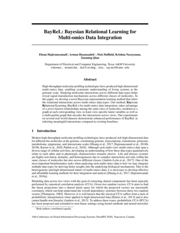
Negative Accuracy1.11.00.90.80.70.60.50.4g Pseudomonasg Pseudomonas s fragig Pseudomonasg Pseudomonas s veroniiAnaerobic microbesPseudomonas metabolites0.25 0.50 0.75 1.00Positive AccuracyFigure 2: Left: Distribution of positive and negative accuracy in different training epochs for BayReLon CF dataset. Right: A sub-network of dependency graph consisting of P. aeruginosa micorbes,their validated targets, and anaerobic microbes, inferred using BayReL.Data description. CF microbiome community within human lungs has been shown to be effected byaltering the chemical environment [Quinn et al., 2015]. Anaerobes and pathogens, two major groupsof microbes, dominate CF. While anaerobes dominate in low oxygen and low pH environments,pathogens, in particular P. aeruginosa, dominate in the opposite conditions [Morton et al., 2019]. Thedataset includes 16S ribosomal RNA (rRNA) sequencing and metabolomics for 172 patients withCF. Following Morton et al. [2019], we filter out microbes that appear in less than ten samples, dueto the overwhelming sparsity of microbiome data, resulting in 138 unique microbial taxa and 462metabolite features. We use the reported target molecules of P. aeruginosa in studies Quinn et al.[2015] and Morton et al. [2019] as a validation set for the microbiome-metabolome interactions.Experimental details and evaluation metrics. We first construct the microbiome and metabolomicnetworks based on their taxonomies and compound names, respectively. For the microbiome network,we perform a taxonomic enrichment analysis using Fisher’s test and calculate p-values for each pairsof microbes. The Benjamini-Hochberg procedure [Benjamini and Hochberg, 1995] is adopted formultiple test correction and an edge is added between two microbes if the adjusted p-value is lowerthan 0.01, resulting in 984 edges in total. The graph density of the microbiome network is 0.102. Forthe metabolomics network, there are 1185 edges in total, with each edge representing a connectionbetween metabolites via a same chemical construction [Morton et al., 2019]. The graph density ofthe metabolite network is 0.011.We evaluate BayReL and baselines in two metrics – 1) accuracy to identify the validated moleculesinteracting with P. aeruginosa which will be referred as positive accuracy, 2) accuracy of not detectingcommon targets between anaerobic microbes and notable pathogen which we refer to this measureas negative accuracy. More specifically, we do not expect any common metabolite targets betweenknown anaerobic microbes (Veillonella, Fusobacterium, Prevotella, and Streptococcus) and notablepathogen P. aeruginosa. If a metabolite molecule x is associated with an anaerobic microbe y, then xis more likely not to be associated with pathogen P. aeruginosa and vice versa. More formally, giventwo disjointPPsets ofPmetabolites s1 and s2 and the set of all microbes T negative accuracy is defined as1(i and j are connected to k)1 i s1 j s2 sk T, where 1(·) is an indicator function. Higher negative1 s2 T accuracy is better as there are fewer common targets between two sets of microbiomes.Numerical results. Considering higher than 97% negative accuracy, the best positive accuracy ofBayReL, BCCA, MOFA, and SRCA are 82.7% 4.7, 28.30% 3.21, 28.13% 3.11, and 26.41%,respectively. Clearly, BayReL substantially outperforms the baselines with up to 54% margin. Thisshows that BayReL not only infers meaningful interactions with high accuracy, but also identifymeicrobiome-metabolite pairs that should not interact. The performance of MOFA is very close toBCCA as expected. This is due to their similar mathematical formulations.We also plot the distribution of positive and negative accuracy in different training epochs for BayReL(Figure 2). We can see that the mass is concentrated on the top right corner, indicating that BayReLconsistently generates accurate interactions in the inferred bipartite graph. Figure 2 also shows6
a sub-network of the inferred bipartite graph consisting P. aeruginosa, anaerobic microbes, andvalidated target nodes of P. aeruginosa and all of the inferred interactions by BayReL between them.While 78% of the validated edges of P. aeruginosa are identified by BayReL, it did not identifyany connection between validated targets of P. aeruginosa and anaerobic microbes, i.e. negativeaccuracy of 100%. However, BCCA at negative accuracy of 100% could identify only one of thesevalidated interactions. This clearly shows the effectiveness and interpretability of BayReL to identifyinter-interactions.When checking the top ten microbiome-metabolite interactions based on the predicted interactionprobabilities, we find that four of them have been reported in other studies investigating CF. Amongthem, microbiome Bifidobacterium, marker of a healthy gut microbiota, has been qPCR validatedto be less abundant in CF patients [Miragoli et al., 2017]. Actinobacillus and capnocytophaga,are commonly detected by molecular methods in CF respiratory secretions [Bevivino et al., 2019].Significant decreases in the proportions of Dialister has been reported in CF patients receiving PPItherapy [Burke et al., 2017].4.2miRNA-mRNA interactions in breast cancerWe further validate whether BayReL can identify potential microRNA (miRNA)-mRNA interactionscontributing to pathogenesis of breast cancer, by integrating miRNA expression with RNA sequencing(RNA-Seq) data from The Cancer Genome Atlas (TCGA) dataset [Tomczak et al., 2015].Data description. It has been shown that miRNAs play critical roles in regulating genes in cellproliferation [Skok et al., 2019, Meng et al., 2015]. To identify miRNA-mRNA interactions thathave a combined effect on a cancer pathogenesis, we conduct an integrative analysis of miRNAexpressions with the consequential alteration of expression profiles in target mRNAs. The TCGAdata contains both miRNA and gene expression data for 1156 breast cancer (BRCA) tumor patients.For RNA-Seq data, we filter out the genes with low expression, requiring each gene to have at least10 count per million in at least 25% of the samples, resulting in 11872 genes for our analysis. Wefurther remove the sequencing depth effect using edgeR [Robinson et al., 2010]. For miRNA data,we have the expression data of 432 miRNAs in total.Experimental details and evaluation metTable 1: Comparison of prediction sensitivity (inrics. To take into account mRNA-mRNA and%) in TCGA for different graph densities.miRNA-miRNA interactions due to their inBCCABayReLvolved roles in tumorigenesis, we construct a Avg. deg. SRCAgene regulatory network (GRN) based on pub0.217.58 21.08 0.0 34.06 2.5licly available BRCA expression data from Clin28.26 31.18 0.7 47.46 2.60.3ical Proteomic Tumor Analysis Consortium (CP0.437.55 41.12 0.2 59.50 3.0TAC) using the R package GENIE3 [Vân AnhHuynh-Thu et al., 2010]. For the miRNAmiRNA interaction networks, we construct a weighted network based on the functional similaritybetween pairs of miRNAs using MISIM v2.0 [Li et al., 2019]. We used miRNA-mRNA interactionsreported by miRNet [Fan and Xia, 2018] as validation set. We calculate prediction sensitivity ofinteractions among validated ones while tracking the average density of the overall constructed graphs.We note that predicting meaningful interactions while inferring sparse graphs is more desirable as theinteractions are generally sparse.Numerical results. The results for prediction sensitivity (i.e. true positive rate) of BayReL andbaselines with different average node degrees based on the interaction probabilities in the inferredbipartite graph are reported in Table 1. As we can see, BayReL outperforms baselines by a largemargin in all settings. With the increasing average node degree (i.e. more dense bipartite graph), theimprovement in sensitivity is more substantial for BayReL. For this dataset, the prediction sensitivityof MOFA (in %) is 22.09, 32.95, and 42.17 for the average degree 0.2, 0.3, and 0.4, respectively. Itslightly outperforms BCCA due to better modeling of RNA-seq count data.We also investigate the robustness of BayReL and BCCA to the number of training samples. Table 2shows the prediction sensitivity of both models while using different percentage of samples to trainthe models. Using 50% of all the samples, while the average prediction sensitivity of BayReL reducesless than 2% in the worst case scenario (i.e. average node density 0.20), BCCA’s performancedegraded around 6%. This clearly shows the robustness of BayReL to the number of training samples.7
In addition, we compare BayReL and BCCA in terms of consistency of identifying significantmiRNA-mRNA interactions as well. We leave out 75% and 50% of all samples to infer the bipartitegraphs, and then compare them with the identified miRNA-mRNA interactions using all of thesamples. The KL divergence values between two inferred bipartite graphs for BayReL are 0.35 and0.32 when using 25% and 50% of samples, respectively. The KL divergence values for BCCA are0.67 and 0.62, using 25% and 50% of samples, respectively. The results prove that BayReL performsbetter than BCCA with fewer number of observed samples.To further show the interpretability of BayReL, we inspect the top inferred interactions. Within them,multiple miRNAs appeared repeatedly. One of them is mir-155 which has been shown to regulatecell survival, growth, and chemosensitivity by targeting FOXO3 in breast cancer [Kong et al., 2010].Another identified miRNA is mir-148b which has been reported as the biomarker for breast cancerprognosis [Shen et al., 2014].4.3Precision medicine in acute myeloid leukemiaWe apply BayReL to identify molecular markers for targeted treatment of acute myeloid leukemia(AML) by integrating gene expression profiles and in vitro sensitivity of tumor samples to chemotherapy drugs with multi-omics prior information incorporated.Classical multi-omics data integration to identify all gene markers of each drug faces several challenges. First, compared to the number of involved molecules and system complexity, the number ofavailable samples for studying complex disease, such as cancer, is often limited, especially considering disease heterogeneity. Second, due to the many biological and experimental confounders, drugresponse could be associated with gene expressions that do not reflect the underlying
heterogeneity and high-dimensional nature of multi-omics data, it is necessary to develop effective and affordable learning methods for their integration and analysis [Huang et al., 2017, Hajiramezanali et al., 2018a]. Modeling data across two views with the goal of extracting shared components has been typically