WIXLIB

Lecture 11Bayesian Modeling (Part 1)(Based on slides by Dr. Tom Rainforth, HT 2020)Jiarui Ganjiarui.gan@cs.ox.ac.uk

Last Lecture: the Bayesian Pipeline

Last Lecture: Bayes’ RuleLikelihoodPrior𝑝 𝐴 𝐵 % 𝑝(𝐵)𝑝 𝐵𝐴 𝑝 𝐴PosteriorEvidence*Image Credit: Paul Epps

Last Lecture: Coin Flipping Example𝑝 𝐻 𝑏𝑖𝑎𝑠𝑒𝑑) 0.2𝑝 𝑇 𝑏𝑖𝑎𝑠𝑒𝑑) 0.8prior belief𝑝 𝑏𝑖𝑎𝑠𝑒𝑑 0.7𝑝 𝑓𝑎𝑖𝑟 0.3biased 0.36!.# !.%𝑝 𝑏𝑖𝑎𝑠𝑒𝑑 𝐻 !.# !.%&!.' !.( 0.48𝑝 𝐻 𝑓𝑎𝑖𝑟) 0.5𝑝 𝑇 𝑓𝑎𝑖𝑟) 0.5𝐻fair𝑝 𝐻 𝐻 𝑝 𝐻 𝑏𝑖𝑎𝑠𝑒𝑑 1 𝑝 𝑏𝑖𝑎𝑠𝑒𝑑 𝐻 𝑝 𝐻 𝑓𝑎𝑖𝑟 1 𝑝 𝑓𝑎𝑖𝑟 𝐻!.' !.(𝑝 𝑓𝑎𝑖𝑟 𝐻 !.# !.%&!.' !.( 0.52

Outline of This Lecture What is a Bayesian model? Bayesian modeling through the eyes of multiple hypotheses Example: Bayesian linear regression

What is a Bayesian Model?

What is a Model? Models are mechanisms for reasoningabout the worldParticle physicsNuclear physicsWeatherMaterial design E.g. Newtonian mechanics, simulators,internal models our brain constructs Good models balance fidelity, predictivepower and tractability- E.g. Quantum mechanics is a moreaccurate model than Newtonianmechanics, but it is actually lessuseful for everyday tasksDrug discoveryCosmology

Example Model: Poler Players’ Reasoning about Each Other

What is a Bayesian Model?A probabilistic generative model 𝑝(𝜃, 𝒟) over latents 𝜃 and data𝒟 It forms a probabilistic “simulator” for generating data that we might haveseen Almost any stochastic simulator can be used as a Bayesian model (we willreturn to this idea in more detail when we cover probabilisticprogramming)

Example Bayesian Model: Captcha Simulator𝑝(letters image)𝑝(image letters)

Example Bayesian Model: Gaussian Mixture Model

Example Bayesian Model: Gaussian Mixture ModelGaussian 1:𝜇! [ 3, 3], Σ! Gaussian 2:𝜇" [3,3], Σ" 1 0.7 0.711 00 1Generative mode:𝜃 Categorical 0.5, 0.5𝑥 𝒩(𝜇# , Σ# )𝑝 𝒟 𝜃 !"# 𝑝(𝑥! 𝜃)

A Fundamental Assumption An assumption made by virtually all Bayesian models is that data points areconditionally independent given the parameter values. In other words, if our data is given by 𝒟 𝑥!likelihood factorizes as: !"# ,we assume that the,𝑝 𝒟 𝜃 5 𝑝(𝑥) 𝜃))* Effectively equates to assuming that our model captures all informationrelevant to prediction For more details, see the lecture notes

“All models are wrong,but some are useful”George Box(1919—2013)

“All models are wrong, but some are useful” The purpose of a model is to help provide insights into a target problem ordata and sometimes to further use these insights to make predictions Its purpose is not to try and fully encapsulate the “true” generative processor perfectly describe the data There are infinite different ways to generate any given dataset. Trying touncover the “true” generative process is not even a well-defined problem In any real–world scenario, no Bayesian model can be “correct”. Theposterior is inherently subjective It is still important to criticize—models can be very wrong! E.g. we can usefrequentist methods to falsify the likelihood

Bayesian ModelingThrough the Eyes ofMultiple Hypotheses

Bayesian Modeling as Multiple HypothesesBayesian models are rooted in hypotheses: Each instance of our parameters 𝜃 is a hypothesis. Given a 𝜃, we cansimulate data using the likelihood model 𝑝(𝐷 𝜃) Bayesian inference allows us to reason about these hypothesis, givingthe probability that each is true given the actual data we observe The posterior predictive is a weighted sum of the predictions from allpossible hypotheses, where these weights are how likely thathypothesis is to be true

Recap: Coin FlippingPosterior predictiveHypotheses𝑝 𝐻 𝑏𝑖𝑎𝑠𝑒𝑑) 0.2𝑝 𝑇 𝑏𝑖𝑎𝑠𝑒𝑑) 0.8prior belief𝑝 𝑏𝑖𝑎𝑠𝑒𝑑 0.7𝑝 𝑓𝑎𝑖𝑟 0.3biased 0.36!.# !.%𝑝 𝑏𝑖𝑎𝑠𝑒𝑑 𝐻 !.# !.%&!.' !.( 0.48𝑝 𝐻 𝑓𝑎𝑖𝑟) 0.5𝑝 𝑇 𝑓𝑎𝑖𝑟) 0.5𝐻fair𝑝 𝐻 𝐻 𝑝 𝐻 𝑏𝑖𝑎𝑠𝑒𝑑 1 𝑝 𝑏𝑖𝑎𝑠𝑒𝑑 𝐻 𝑝 𝐻 𝑓𝑎𝑖𝑟 1 𝑝 𝑓𝑎𝑖𝑟 𝐻!.' !.(𝑝 𝑓𝑎𝑖𝑟 𝐻 !.# !.%&!.' !.( 0.52Posterior

Example: Density Estimation Suppose that we decide to use an isotropicGaussian likelihood with unknown mean 𝜃to model the data on the right:where 𝐼 is a two-dimensional identitymatrix

Example: Density EstimationHypothesis 1: 𝜃 2, 0𝑝 𝒟 𝜃 2,0 0.00059 10"%

Example: Density EstimationHypothesis 1: 𝜃 2, 0𝑝 𝒟 𝜃 2,0 0.00059 10"%Hypothesis 2: 𝜃 0, 0𝑝 𝒟 𝜃 0,0 0.99 10"%

Example: Density EstimationHypothesis 1: 𝜃 2, 0𝑝 𝒟 𝜃 2,0 0.00059 10"%Highest likelihoodHypothesis 2: 𝜃 0, 0𝑝 𝒟 𝜃 0,0 0.99 10"%Hypothesis 3: 𝜃 2, 0𝑝 𝒟 𝜃 2,0 0.021 10"%

The Posterior Predictive Averages over Hypotheses (1) The posterior predictive distribution allows us to average over each of ourhypotheses, weighting each by their posterior probability. For example, in our density estimation example, lets introduce (the ratherunusual but demonstrative) prior:

The Posterior Predictive Averages over Hypotheses (2) Then we have:

The Posterior Predictive Averages over Hypotheses (3) Inserting our likelihoods from earlier and trawling through the algebra givesWe thus have that the posterior predictive is a weighted sum of the threepossible predictive distributions

The Posterior Predictive Averages over Hypotheses

Some Subtleties Even though we average over 𝜃, a Bayesian model is still implicitly assuming thatthere is still a single true 𝜃- The averaging over hypotheses is from our own uncertainty as which one is correct- This can be problematic with lots of data given our model is an approximation In the limit of large data, the posterior is guaranteed to collapse to a point estimate:𝑝(𝜃 𝑥 :, ) 𝛿 𝜃 𝜃 as 𝑁 The value of 𝜃 and the exact nature of this convergence is dictated by theBernstein–von Mises Theorem (see the lecture notes) Note that, subject to mild assumptions, 𝜃 is independent of the prior: with enoughdata, the likelihood always dominates the prior

Example:Bayesian Linear Regression

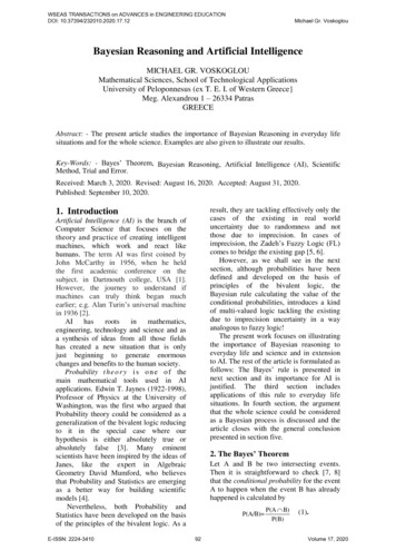
Linear RegressionHouse size is a good linear predictor for price (ignore the colors) Learn a function that maps size to price

Linear Regression Inputs: 𝑥 ℝ. (where 𝐷 1 for this example) Outputs: 𝑦 ℝ Data: 𝐷 𝑥) , 𝑦),)/ Regression model: 𝑦 𝑥 0𝑤 𝑏 where 𝑤 ℝ. and 𝑏 ℝWe can simplify this notation by redefining 𝑥 1, 𝑥 0that the model becomes 𝑦 𝑥 0𝑤0and 𝑤 𝑏, 𝑤 0 0, soClassical least squares linear regression is a discriminative method aiming tominimize the empirical mean squared error𝐿(𝑤) , , )/ #0𝑦) 𝑥) 𝑤

Linear Regression*Image credit: Pier Palamara

Bayesian Linear Regression Least square provides a point estimate without uncertaintyw argmin 𝐿(𝑤)& Bayesian method introduces uncertainty by building a probabilisticgeneric model based around linear regression and then beingBayesian about the weights

Bayesian Linear Regression: Prior and Likelihood For example, prior of 𝑤 is a zero-meanGaussian with a fixed covariance 𝐶𝑝 𝑤 𝒩(𝑤; 0, 𝐶) And given input 𝑥, the output is 𝑦 𝑥 0𝑤plus a Gaussian noise, and datapoints areindependent of each other:𝑝 𝑦 𝑥, 𝑤 ,)/ 𝑝(𝑦) 𝑥) , 𝑤) 0# ,)/ 𝒩(𝑦) ; 𝑥) 𝑤, 𝜎 )where 𝜎 is a fixed standard deviation*Image credit: Roger Grosse

Bayesian Linear Regression: Posterior Using Bayes’ rule (and some math) to derive the posterior. See Bishop, Patternrecognition and machine learning, 2006, Chapter 3

Bayesian Linear Regression: Posterior Note here that the fact the prior and posterior share the same form is highlyspecial case. This is known as a conjugate distribution and it is why we were ableto find an analytic solution for the posterior.Posterior after 1 observationPosterior after 2 observations

Bayesian Linear Regression: Posterior*Bishop, Pattern recognition and machine learning.

Bayesian Linear Regression: Posterior*Bishop, Pattern recognition and machine learning.

Bayesian Linear Regression: Posterior Predictive Some more math to derive the posterior predictive where the result is again aconsequence of Gaussian identities, and 𝑚 and 𝑆 are as before

Bayesian Linear Regression: Posterior Predictive*Image credit: https://www.dataminingapps.com/2017/09/simple- linear- regression- do- it- the- bayesian- way/

Further Reading Information on non-parametric models and Gaussian processes in course notes Bishop, Pattern recognition and machine learning, Chapters 1-3 K P Murphy. Machine learning: a probabilistic perspective. 2012, Chapter 5 D Barber. Bayesian reasoning and machine learning. 2012, Chapter 12 T P Minka. “Bayesian model averaging is not model combination”. In: (2000) Zoubin Ghahramani on Bayesian machine learning (there are various alternativevariations of this talk): https://www.youtube.com/watch?v y0FgHOQhG4w Iain Murray on Probabilistic Modeling https://www.youtube.com/watch?v pOtvyVYAuW4

Machine learning: a probabilistic perspective. 2012, Chapter 5 D Barber. Bayesian reasoning and machine learning. 2012, Chapter 12 T P Minka. "Bayesian model averaging is not model combination". In: (2000) ZoubinGhahramanion Bayesian machine learning (there are various alternative