Transcription
Module 4: Chapter 6Bayesian Learning
1. Introduction A probabilistic approach to inference It is based on the assumption that the quantities ofinterest are governed by probability distributions andthat optimal decisions can be made by reasoning aboutthese probabilities together with observed data.
Quantitative approach to weighing the evidencesupporting alternative hypotheses Important Calculates the explicit probability like naïve Bayes. Naive Bayes classifier competitive, outperforms as aclassifier They help Understand learning algorithms that donot explicitly manipulate probabilities
4Machine Learning15CS7317-10-2019 Bayesian learning methods are relevant to our study of machinelearning for two different reasons.i.Bayesian learning algorithms that calculate explicitprobabilities for hypotheses, such as the naive Bayesclassifier, are among the most practical approaches tocertain types of learning problems.
5 For ex : Michie et al.(1994) provide a detailed studycomparing the naive Bayes classifier to other learningalgorithms, including decision tree and neural networkalgorithms.Machine Learning15CS7317-10-2019 These researchers show that the naive Bayes classifier iscompetitive with these other learning algorithms in manycases and that in some cases it outperforms these othermethods.ii. The Bayesian methods are important to our study ofmachine learning is that they provide a useful perspectivefor understanding many learning algorithms that do notexplicitly manipulate probabilities.
6 For ex : We will analyze the algorithms such as the FINDS and Candidate-Elimination algorithms to determine theconditions under which they output the most probablehypothesis given the training data.Machine Learning15CS7317-10-2019 Bayesian analysis provides an opportunity for thechoosing the appropriate alternative error function(crossentropy) in neural network learning algorithms. We use a Bayesian perspective to analyze the inductivebias of decision tree learning algorithms that favor shortdecision trees and examine the closely related MinimumDescription Length principle.
Feature of Bayesian learning methodsinclude: Each observed training example can incrementally decrease orincrease the estimated probability that a hypothesis is correct. Thisprovides a more flexible approach to the learning compared to thealgorithms that completely eliminate a hypothesis if it is found tobe inconsistent with any single example. Prior knowledge can be combined with observed data to determinethe final probability of a hypothesis. The prior probability is gotthrough (i) a prior probability of each candidate hypothesis (ii) aprobability distribution over observed data for each possiblehypothesis. Bayesian methods can accommodate hypotheses that makeprobabilistic predictions For ex : hypotheses such as “thispneumonia patient has a 93% chance of complete recovery”
New instances can be classified by combining thepredictions of multiple hypotheses, weighted by theirprobabilities. Even in cases where Bayesian methods provecomputationally intractable, they can provide astandard of optimal decision making against whichother practical methods can be measured.
Difficulty of applying Bayesian method Bayesian methods typically require initial knowledge of manyprobabilities. The significant computational cost required to determine theBayes optimal hypothesis in the general case.
2. BAYES THEOREM Determining the most (best) hypothesis from somespace H, (having initial prior probabilities of varioushypotheses ) given the observed training data D. Calculates the probability of a hypothesis based on itsprior probability, the probabilities of observingvarious data given the hypothesis, and the observeddata itself.
Notation P(h) : initial probability that hypothesis h holds, beforewe have observed the training data. prior probabilityof h and may reflect any background knowledge we haveabout the chance that h is a correct hypothesis. P(D) : prior probability that training data D will beobserved-no knowledge of h P(D h) : probability of observing data D in whichhypothesis h holds. P(h D) : probability that h holds given the observedtraining data D. posterior probability of h reflectsthe influence of the training data D
The learner considers some set of candidatehypotheses H and is interested in finding themost probable hypothesis h ϵ H given theobserved data D (or at least one of themaximally probable if there are several). Any such maximally probable hypothesis iscalled a maximum a posteriori (MAP)hypothesis
We can determine the MAP hypotheses by usingBayes theorem to calculate the posteriorprobability of each candidate hypothesis.
hMAP is a MAP hypothesis provided
In some cases, we will assume that everyhypothesis in H is equally probable a priori(P(hi) P(hj) for all hi and hj in H). In this case we can further simplify Equationand need only consider the term P(D h) to findthe most probable hypothesis
P(D h) is often called the likelihood of the data D given h Any hypothesis that maximizes P(D h) is called amaximum likelihood (ML) hypothesis, hML.
Example: To illustrate Bayes rule, consider a medicaldiagnosis problem in which there are twoalternative hypotheses:(1) that the patient has a particular form of cancer(2) that the patient does not.
The available data is from a particular laboratory testwith two possible outcomes: (positive) and (negative). We have prior knowledge that over the entire populationof people only .008 have this disease. Furthermore, the lab test is only an imperfect indicatorof the disease. The test returns a correct positive result in only 98% ofthe cases in which the disease is actually present and acorrect negative result in only 97% of the cases in whichthe disease is not present. In other cases, the test returns the opposite result.
Suppose we now observe a new patient for whom the labtest returns a positive result. Should we diagnose the patient as having cancer or not?
3. BAYESLEARNINGTHEOREMANDCONCEPT What is the relationship between Bayes theorem and theproblem of concept learning? Bayes theorem provides a principled way to calculate theposterior probability of each hypothesis given thetraining data we can use it as the basis for a straightforwardlearning algorithm that calculates the probability foreach possible hypothesis then outputs the most probable.
3.1 Brute-Force Bayes ConceptLearning
Concept learning problem: assume the learner considers some finite hypothesis spaceH defined over the instance space X, the task is to learn some target concept c : X - {0,1}. learner is given some sequence of training examples((x1,d1 ). . . (xm, dm))
We can design a straightforward conceptlearning algorithm to output the maximum aposteriori hypothesis, based on Bayes theorem.
BRUTE-FORCE MAP LEARNING algorithm
what values are to be used for P(h) and for P(D h) ? choose the probability distributions P(h) and P(D h) inany way you wish, to describe our prior knowledgeabout the learning task. Here let us choose them to be consistent with thefollowing assumptions:1. The training data D is noise free (i.e., di c(xi)).2. The target concept c is contained in the hypothesisspace H3. We have no a priori reason to believe that anyhypothesis is more probable than any other.
Given these assumptions, what values should wespecify for P(h)? Given no prior knowledge that one hypothesis ismore likely than another, it is reasonable to assignthe same prior probability to every hypothesis hin H. because we assume the target concept is containedin H we should require that these priorprobabilities sum to 1.
Together these constraints imply that we shouldchoose
What choice shall we make for P(D h)? P(D h) is the probability of observing the targetvalues D (d1 . . dm) for the fixed set of instances (x1. . . xm), given a world in which hypothesis h holds(i.e., given a world in which h is the correct descriptionof the target concept c).
Since we assume noise-free training data, theprobability of observing classification di , givenh is 1 if di h(xi) and 0 if di h(xi)
In other words, the probability of data D given hypothesis h is 1 if D isconsistent with h, and 0 otherwise.
Given these choices for P(h) and for P(D h) we nowhave a fully-defined problem for the above BRUTEFORCE MAP LEARNING algorithm.
Step1 : Let us consider the first step of this algorithm,which uses Bayes theorem to compute theposterior probability P(h D) of each hypothesis hgiven the observed training data D.
Case 1 : h is inconsistent with the training data D.The posterior probability of a hypothesis inconsistent with D iszero.
Case 2: h is consistent with D.
The above analysis implies that under our choice for P(h)and P(D h), every consistent hypothesis has posteriorprobability (1 / VSH,D ), and every inconsistenthypothesis has posterior probability 0. Every consistent hypothesis is, therefore, a MAPhypothesis.
3.2 MAPLearnersHypothesesandConsistent Every hypothesis consistent with D is a MAPhypothesis
consistent learners: We will say that a learning algorithm is a consistentlearner provided it outputs a hypothesis that commitszero errors over the training examples. Given the above analysis, we can conclude that everyconsistent learner outputs a MAP hypothesis, if weassume a uniform prior probability distribution over H (i.e., P(hi) P(hj) for all i, j), and deterministic, noise free training data (i.e., P(D h) 1 if Dand h are consistent, and 0 otherwise).
4. MAXIMUM LIKELIHOOD AND LEASTSQUARED ERROR HYPOTHESES Let’s we consider the problem of learning acontinuous-valued target function.
A straightforward Bayesian analysis will showthat under certain assumptions anylearning algorithm that minimizes thesquared error between the outputhypothesis predictions and the trainingdata will output a maximum likelihoodhypothesis.
Consider the following problem setting: Learner L considers an instance space X and ahypothesis space H consisting of some class ofreal-valued functions defined over X (i.e., each hin H is a function of the form h : X R, where Rrepresents the set of real numbers).
The problem faced by L is to learn an unknowntarget function f : X R drawn from H. A set of m training examples is provided, wherethe target value of each example is corrupted byrandom noise drawn according to a Normalprobability distribution.
More precisely, each training example is a pairof the form (xi, di) wheredi f (xi) ei f(xi) : the noise-free value of the target function ei: is a random variable representing the noise.
It is assumed that the values of the ei are drawnindependently and that they are distributedaccording to a Normal distribution withzero mean. The task of the learner is to output a maximumlikelihood hypothesis, or, equivalently, a MAPhypothesis assuming all hypotheses are equallyprobable a priori.
2 basic concepts probability densities Normal distributions.
First, in order to discuss probabilities overcontinuous variables such as e,we mustintroduce probability densities. The reason, roughly, is that we wish for the totalprobability over all possible values of therandom variable to sum to one.
In the case of continuous variables we cannotachieve this by assigning a finite probability toeach of the infinite set of possible values for therandom variable. Instead, we speak of a probability density forcontinuous variables such as e and require thatthe integral of this probability density over allpossible values be one.
Second, we stated that the random noisevariable e is generated by a Normal probabilitydistribution. A Normal distribution is a smooth, bell-shapeddistribution that can be completely characterizedby its mean μ and its standard deviation σ.
Given this background we now return to themain issue: showing that the least-squared error hypothesis is,in fact, the maximum likelihood hypothesis withinour problem setting. We will show this by deriving the maximumlikelihood hypothesis, but using lower case p torefer to the probability density
we assume a fixed set of training instances (x1, x2 . . . xm)and Therefore consider the data D to be the correspondingsequence of target values D ( d1, d2 . . .dm). Here di f (xi) ei.
Assuming the training examples are mutuallyindependent given h, we can write P(D h) as the product of the variousp(di h)
Given that the noise ei obeys a Normal distribution withzero mean and unknown variance σ2 , each di must alsoobey a Normal distribution with variance σ2 centeredaround the true target value f(xi) rather than zero. Therefore p(di h) can be written as a Normaldistribution with variance σ2 and mean μ f (xi)
Thus, Equation shows that the maximumlikelihood hypothesis hML is the one thatminimizes the sum of the squared errorsbetween the observed training values di and thehypothesis predictions h(xi).
Limitations of this problem setting. The above analysis considers noise only in thetarget value of the training example and doesnot consider noise in the attributes describingthe instances themselves.
Machine Learning-Module 411-11-2019Machine Learning-15CS731
Chapter 6: Bayesian LearningIntroduction Bayesian reasoning provides a probabilistic approach toinference. Bayesian learning methods are relevant to our study of machinelearning for two different reasons.i.11-11-2019Bayesian learning algorithms that calculate explicitprobabilities for hypotheses, such as the naive Bayesclassifier, are among the most practical approaches tocertain types of learning problems.Machine Learning-15CS732
For ex : Michie et al.(1994) provide a detailed studycomparing the naive Bayes classifier to other learningalgorithms, including decision tree and neural networkalgorithms. These researchers show that the naive Bayes classifier iscompetitive with these other learning algorithms in manycases and that in some cases it outperforms these othermethods.ii. The Bayesian methods are important to our study ofmachine learning is that they provide a useful perspectivefor understanding many learning algorithms that do notexplicitly manipulate probabilities.11-11-2019Machine Learning-15CS733
For ex : We will analyze the algorithms such as the FINDS and Candidate-Elimination algorithms to determine theconditions under which they output the most probablehypothesis given the training data. Bayesian analysis provides an opportunity for thechoosing the appropriate alternative error function(crossentropy) in neural network learning algorithms. We use a Bayesian perspective to analyze the inductivebias of decision tree learning algorithms that favor shortdecision trees and examine the closely related MinimumDescription Length principle.11-11-2019Machine Learning-15CS734
Features of Bayesian Learning methods Each observed training example can incrementally decrease orincrease the estimated probability that a hypothesis is correct.This provides a more flexible approach to the learning comparedto the algorithms that completely eliminate a hypothesis if it isfound to be inconsistent with any single example. Prior knowledge can be combined with observed data todetermine the final probability of a hypothesis. The priorprobability is got through (i) a prior probability of each candidatehypothesis (ii) a probability distribution over observed data foreach possible hypothesis. Bayesian methods can accommodate hypotheses that makeprobabilistic predictions For ex : hypotheses such as “thispneumonia patient has a 93% chance of complete recovery”11-11-2019Machine Learning-15CS735
New instances can be classified by combining the predictions ofmultiple hypotheses, weighted by their probabilities. Even in cases where Bayesian methods prove computationallyintractable, they can provide a standard of optimal decision makingagainst which other practical methods can be measured.Practical Difficulties in applying Bayesian Methods Bayesian methods typically require initial knowledge of manyprobabilities. The significant computational cost required to determine the Bayesoptimal hypothesis in the general case.11-11-2019Machine Learning-15CS736
Bayes Theorem In machine learning we are interested in determining the besthypothesis from some space H, given the observed training data D. Bayes theorem provides a way to calculate the probability of ahypothesis based on its prior probability, the probabilities ofobserving various data given the hypothesis, and the observed dataitself. To define Bayes theorem precisely, let us define the followingnotations P(h) denote the initial probability or prior probability thathypothesis h holds. P(D) – denote the prior probability that training data D will beobserved.11-11-2019Machine Learning-15CS737
P(D/h) denote the probability of observing data D given someworld in which hypothesis h holds. P(h/D) denote the posterior probability of h because itreflects our confidence that h holds after we haveseen the training data D. Bayes theorem is the cornerstone of Bayesian learning methodsbecause it provides a way to calculate the posterior probabilityP(h/D) from the prior probability P(h), together with P(D) andP(D/h)𝑷 𝒉/𝑫 𝑷 𝑫/𝒉 𝑷(𝒉)𝑷(𝑫)Eqn 6.1 P(h/D) increases with P(h) and with P(D/h) according to Bayestheorem.11-11-2019Machine Learning-15CS738
It is also reasonable to see that P(h/D) decreases as P(D) increases,because the more probable it is that D will be observedindependent of h, the less evidence D provides in support of h. In many learning scenarios, the learner considers some set ofcandidate hypotheses H and is interested in finding the mostprobable hypothesis h H given the observed data D. Any such maximally probable hypothesis is called a maximum aposteriori (MAP) hypothesis. We can determine the MAP hypotheses by using Bayes theorem tocalculate the posterior probability of each candidate hypothesis. More precisely, we will say that hMAP is a MAP hypothesisprovided:11-11-2019Machine Learning-15CS739
Eqn 6.2 Notice in the final step above we dropped the term P(D) because itis a constant independent of h. In some cases, we will assume that every hypothesis in H is equallyprobable a priori (P(hi) P(hj) for all hi and hj in H). In this casewe can further simplify Eqn 6.2 and need only consider the termP(D/h) to find the most probable hypothesis.11-11-2019Machine Learning-15CS7310
P(D/h) is often called the likelihood of the data D given h, and anyhypothesis that maximizes P(D/h) is called a maximum likelihood(ML) hypothesis, hMLEqn 6.3 In order to make clear the connection to machine learningproblems, we have learnt Bayes theorem above by referring to thedata D as training examples of some target function and referring toH as the space of candidate target functions.11-11-2019Machine Learning-15CS7311
An Example To illustrate Bayes rule, consider a medical diagnosis problem inwhich there are two alternative hypotheses:i. that the patient has a particular form of cancerii. that the patient does not The available data is from a particular laboratory test with twopossible outcomes: (positive) and (negative). We have prior knowledge that over the entire population of peopleonly .008 have this disease. The test returns a correct positive result in only 98% of the cases inwhich the disease is actually present and a correct negative result inonly 97% of the cases in which the disease is not present.11-11-2019Machine Learning-15CS7312
In other cases, the test returns the opposite result. The above situation can be summarized by the followingprobabilities: Suppose we now observe a new patient for whom the lab testreturns a positive result. Should we diagnose the patient as havingcancer or not? The maximum a posteriori hypothesis can be found using Eqn 6.2:P(cancer/ ) P( /cancer) P(cancer) 0.98 * 0.008 0.0078P( cancer/ ) P( / cancer) P( cancer) 0.03* 0.992 0.029811-11-2019Machine Learning-15CS7313
Thus, hMAP cancer Notice that while the posterior probability of cancer is significantlyhigher than its prior probability, the most probable hypothesis isstill that the patient does not have cancer. As this example illustrates, the result of Bayesian inferencedepends strongly on the prior probabilities, which must beavailable in order to apply the method directly. Basic formulas for calculating probabilities are summarized inTable 6.1.11-11-2019Machine Learning-15CS7314
Table 6.1: Summary of basic probability formulas11-11-2019Machine Learning-15CS7315
Bayes Theorem and Concept Learning Consider the concept learning problem in which we assume thatlearner considers some finite hypothesis space H defined over theinstance space X, in which the task is to learn some target conceptc:X {0,1}. Let us assume that the learner is given some sequence of trainingexamples x1,d1 xm,dm where xi is some instance from Xand where di is the target value of xi (i.e., di c(xi)). To understand in very simple way, let us make one moreassumption that the sequence of instances xl . . . xm is heldfixed, so that the training data D can be written simply as thesequence of target values D dl . . . dm .11-11-2019Machine Learning-15CS7316
Thus, we can design a straightforward concept learning algorithmto output the maximum a posteriori hypothesis, based on Bayestheorem, as follows:Brute-Force MAP Learning Algorithm1. For each hypothesis h in H, calculate the posterior probability2. Output the hypothesis hMAP with the highest posterior probabilityThis algorithm may require significant computation, because it appliesBayes theorem to each hypothesis in H to calculate P(h/D).11-11-2019Machine Learning-15CS7317
In order to specify a learning problem for the Brute-force MAPlearning algorithm we must specify what values are to be used forP(h) and for P(D/h). Let us choose them to be consistent with the followingassumptions:i. The training data D is noise free (i.e., di c(xi)).ii. The target concept c is contained in the hypothesis space H.iii. We have no a priori reason to believe that any hypothesis ismore probable than any other. Given these assumptions, we specify the value for P(h) in thefollowing way Given no prior knowledge that one hypothesis is more likelythan another, it is reasonable to assign the same priorprobability to every hypothesis h in H.11-11-2019Machine Learning-15CS7318
Furthermore, because we assume the target concept iscontained in H we should require that these prior probabilitiessum to 1. Together these constraints imply that we should choose The value for P(D/h) can be specified in the following way: P(D/h) is the probability of observing the target values D dl. . .dm for the fixed set of instances x1 . . . xm given a worldin which hypothesis h holds. Since we assume noise-free training data, the probability ofobserving classification di given h is just 1 if di h(xi) and 0 ifdi h(xi)11-11-2019Machine Learning-15CS7319
Therefore,Eqn 6.4 Given these choices for P(h) and for P(D/h) we now have a fullydefined problem for the above Brute-Force MAP learningalgorithm. Now, let us consider the first step of this algorithm, which usesBayes theorem to compute the posterior probability P(h/D) of eachhypothesis h given the observed training data D. Recalling Bayes theorem, we have11-11-2019Machine Learning-15CS7320
Case 1: Consider where h is inconsistent with the training data D Since Eqn 6.4 defines P(D/h) to be 0 when h is inconsistentwith D, we haveThe posterior probability of a hypothesis inconsistent with D iszero. Case 2:Consider the case where h is consistent with D. Since Eqn 6.4 defines P(D/h) to be 1 when h is consistent withD, we have11-11-2019Machine Learning-15CS7321
where VSH,D is the subset of hypotheses from H that are consistentwith D.11-11-2019Machine Learning-15CS7322
Verification It is easy 𝑽𝑺𝑯 𝑫 .of the value P(D) for 𝑯 𝑽𝑺𝑯 𝑫 .to verify that P(D) , 𝑯 concept learningbecause the sum over allhypotheses of P(h/D) must be one and because the number ofhypotheses from H consistent with D is by definition VSH,D Alternatively, we can derive P(D) from the theorem of totalprobability and the fact that the hypotheses are mutually exclusive(i.e., ( i j)(P(hi hj) 0))11-11-2019Machine Learning-15CS7323
To summarize, Bayes theorem implies that the posterior probabilityP(h/D) under our assumed P(h) and P(D/h) isEqn 6.5where VSH,D is the number of hypotheses from H consistent withD. The evolution of probabilities associated with hypotheses isdepicted schematically in figure 6.1. Initially figure 6.1(a) showsall hypotheses have the same probability. As the training dataaccumulates (figure 6.1(b) & figure 6.1(c)) the posterior probabilityfor inconsistent hypotheses becomes zero while the totalprobability summing to one is shared equally among the remainingconsistent hypotheses.11-11-2019Machine Learning-15CS7324
Figure 6.1: Evolution of posterior probabilities P(h/D) with increasing training data11-11-2019Machine Learning-15CS7325
MAP Hypotheses and Consistent Learners Given the above analysis, every consistent learner outputs a MAPhypothesis, if we assume a uniform prior probability distributionover H (i.e., P(hi) P(hj) for all i, j), and if we assumedeterministic, noise free training data (i.e., P(D/h) 1 if D and hare consistent, and 0 otherwise). For ex : Consider the Find-S concept learning algorithm. The Find-Ssearches the hypothesis space H from specific to generalhypotheses, outputting a maximally specific consistenthypothesis. Because FIND-S outputs a consistent hypothesis, we know thatit will output a MAP hypothesis under the probabilitydistributions P(h) and P(D/h) defined.11-11-2019Machine Learning-15CS7326
Actually, FIND-S does not explicitly manipulate probabilitiesat all-it simply outputs a maximally specific member of theversion space. However, by identifying distributions for P(h) and P(D/h)under which its output hypotheses will be MAP hypotheses, wehave a useful way of characterizing the behavior of FIND-S. Are there other probability distributions for P(h) and P(D/h)under which FIND-S outputs MAP hypotheses? Yes. Because FIND-S outputs a maximally specific hypothesisfrom the version space, its output hypothesis will be a MAPhypothesis relative to any prior probability distribution thatfavors more specific hypotheses.11-11-2019Machine Learning-15CS7327
More precisely, suppose H is any probability distribution P(h)over H that assigns P(h1) P(h2) if hl is more specific than h2. Then it can be shown hat FIND-S outputs a MAP hypothesisassuming the prior distribution H and the same distributionP(D/h) To summarize, the Bayesian framework allows one way tocharacterize the behavior of learning algorithms (e.g., FIND-S),even when the learning algorithm does not explicitly manipulateprobabilities.11-11-2019Machine Learning-15CS7328
Definitions of various Probability TermsRandom Variable: A random variable, usually written X, is avariable whose possible values are numerical outcomes of a randomphenomenon.There are two types of random variables, discrete and continuous.For ex : Random variable can be defined for a coin flip as follows𝟏 𝒊𝒇 𝒊𝒕 𝒊𝒔 𝒉𝒆𝒂𝒅X 𝟎 𝒊𝒇 𝒊𝒕 𝒊𝒔 𝒕𝒂𝒊𝒍Discrete Random Variable : The variables which can takedistinct/separate values are called discrete random variables.For ex : Flipping a fair coin, rolling a dice11-11-2019Machine Learning-15CS7329
Continuous Random Variable : The variables which can take anyvalues in a range are called continuous random variables.For ex : Height and Weight of the person, Mass of an animalProbability Distribution : It is a mathematical function that providesthe probabilities of occurrence of different possible outcomes in anexperiment.Constructing a probability distribution for random variable Let us take random variable,X no of heads after 3 flips of a fair coin Then the probability distribution table can be written as follows:11-11-2019Machine Learning-15CS7330
Outcomes(No of Heads)X 0X 1X 2X 3Probability1/83/83/81/811-11-2019Machine Learning-15CS7331
Maximum LikelihoodHypothesesandLeastSquaredError Many learning approaches such as neural network learning, linearregression and polynomial curve fitting will face a problem oflearning a continuous-valued target function. A straightforward Bayesian analysis will show that under certainassumptions any learning algorithm that minimizes the squarederror between the output hypothesis predictions and the trainingdata will output a maximum likelihood hypothesis. Consider the following problem setting. Learner L considers aninstance space X and a hypothesis space H consisting of some classof real-valued functions defined over X. (i.e., each h in H is afunction of the form h:X ℝ, where ℝ represents the set of realnumbers).11-11-2019Machine Learning-15CS7332
The problem faced by L is to learn an unknown target function f :X ℝ drawn from H. A set of m training examples is provided, where the target value ofeach example is corrupted by random noise drawn according to aNormal probability distribution. More precisely, each training example is a pair of the form xi, di where di f (xi) ei. Here f(xi) is the noise-free value of the targetfunction and ei is a random variable representing the noise. It is assumed that the values of the ei are drawn independently andthat they are distributed according to a Normal distribution withzero mean. The task of the learner is to output a maximum likelihoodhypothesis, o
Machine Learning- 17-10-2019 15CS73 4 Bayesian learning methods are relevant to our study of machine learning for two different reasons. i. Bayesian learning algorithms that calculate explicit probabilities for hypotheses, such as the naive Bayes classifier, are among the most practical approaches to certain types of learning problems.


