Transcription
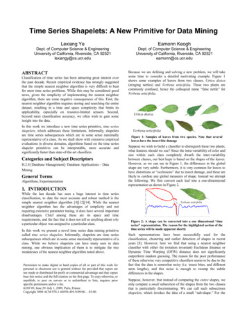
Time Series Shapelets: A New Primitive for Data MiningLexiang YeEamonn KeoghDept. of Computer Science & EngineeringUniversity of California, Riverside, CA 92521lexiangy@cs.ucr.eduDept. of Computer Science & EngineeringUniversity of California, Riverside, CA 92521eamonn@cs.ucr.eduABSTRACTClassification of time series has been attracting great interest overthe past decade. Recent empirical evidence has strongly suggestedthat the simple nearest neighbor algorithm is very difficult to beatfor most time series problems. While this may be considered goodnews, given the simplicity of implementing the nearest neighboralgorithm, there are some negative consequences of this. First, thenearest neighbor algorithm requires storing and searching the entiredataset, resulting in a time and space complexity that limits itsapplicability, especially on resource-limited sensors. Second,beyond mere classification accuracy, we often wish to gain someinsight into the data.In this work we introduce a new time series primitive, time seriesshapelets, which addresses these limitations. Informally, shapeletsare time series subsequences which are in some sense maximallyrepresentative of a class. As we shall show with extensive empiricalevaluations in diverse domains, algorithms based on the time seriesshapelet primitives can be interpretable, more accurate andsignificantly faster than state-of-the-art classifiers.Categories and Subject DescriptorsH.2.8 [Database Management]: Database Applications – DataMiningGeneral TermsAlgorithms, ExperimentationBecause we are defining and solving a new problem, we will takesome time to consider a detailed motivating example. Figure 1shows some examples of leaves from two classes, Urtica dioica(stinging nettles) and Verbena urticifolia. These two plants arecommonly confused, hence the colloquial name “false nettle” forVerbena urticifolia.Urtica dioicaVerbena urticifoliaFigure 1: Samples of leaves from two species. Note that severalleaves have the insect-bite damageSuppose we wish to build a classifier to distinguish these two plants;what features should we use? Since the intra-variability of color andsize within each class completely dwarfs the inter-variabilitybetween classes, our best hope is based on the shapes of the leaves.However, as we can see in Figure 1, the differences in the globalshape are very subtle. Furthermore, it is very common for leaves tohave distortions or “occlusions” due to insect damage, and these arelikely to confuse any global measures of shape. Instead we attemptthe following. We first convert each leaf into a one-dimensionalrepresentation as shown in Figure 2.1. INTRODUCTIONWhile the last decade has seen a huge interest in time seriesclassification, to date the most accurate and robust method is thesimple nearest neighbor algorithm [4][12][14]. While the nearestneighbor algorithm has the advantages of simplicity and notrequiring extensive parameter tuning, it does have several importantdisadvantages. Chief among these are its space and timerequirements, and the fact that it does not tell us anything about whya particular object was assigned to a particular class.In this work we present a novel time series data mining primitivecalled time series shapelets. Informally, shapelets are time seriessubsequences which are in some sense maximally representative of aclass. While we believe shapelets can have many uses in datamining, one obvious implication of them is to mitigate the twoweaknesses of the nearest neighbor algorithm noted above.Permission to make digital or hard copies of all or part of this work forpersonal or classroom use is granted without fee provided that copies arenot made or distributed for profit or commercial advantage and that copiesbear this notice and the full citation on the first page. To copy otherwise, orrepublish, to post on servers or to redistribute to lists, requires priorspecific permission and/or a fee.KDD’09, June 29–July 1, 2009, Paris, FranceCopyright 2009 ACM 978-1-60558-495-9/09/06. 5.00.Verbena urticifoliaFigure 2: A shape can be converted into a one dimensional “timeseries” representation. The reason for the highlighted section of thetime series will be made apparent shortlySuch representations have been successfully used for theclassification, clustering and outlier detection of shapes in recentyears [8]. However, here we find that using a nearest neighborclassifier with either the (rotation invariant) Euclidean distance orDynamic Time Warping (DTW) distance does not significantlyoutperform random guessing. The reason for the poor performanceof these otherwise very competitive classifiers seems to be due to thefact that the data is somewhat noisy (i.e. insect bites, and differentstem lengths), and this noise is enough to swamp the subtledifferences in the shapes.Suppose, however, that instead of comparing the entire shapes, weonly compare a small subsection of the shapes from the two classesthat is particularly discriminating. We can call such subsectionsshapelets, which invokes the idea of a small “sub-shape.” For the
moment we ignore the details of how to formally define shapelets,and how to efficiently compute them. In Figure 3, we see theshapelet discovered by searching the small dataset shown in Figure1.ShapeletThe leaf example, while from an important real-world problem inbotany, is a contrived and small example to help develop thereader’s intuitions. However, as we shall show in Section 5, we canprovide extensive empirical evidence for all of these claims, on avast array of problems in domains as diverse as anthropology,human motion analysis, spectrography, and historical manuscriptmining.2. RELATED WORK AND BACKGROUNDUrtica dioicaVerbena urticifoliaFigure 3: Here, the shapelet hinted at in Figure 2 (in both casesshown with a bold line), is the subsequence that best discriminatesbetween the two classesAs we can see, the shapelet has “discovered” that the definingdifference between the two species is that Urtica dioica has a stemthat connects to the leaf at almost 90 degrees, whereas the stem ofVerbena urticifolia connects to the leaf at a much shallower angle.Having found the shapelet and recorded its distance to the nearestmatching subsequence in all objects in the database, we can buildthe simple decision-tree classifier shown in Figure 4.Shapelet Dictionary5.1I32100Does Q have a subsequence withina distance 5.1 of shape I ?yes0IWhile there is a vast amount of literature on time seriesclassification and mining [4][7][14], we believe that the problem weintend to solve here is unique. The closest work is that of [5]. Herethe author also attempts to find local patterns in a time series whichare predictive of a class. However, the author considers the problemof finding the best such pattern intractable, and thus resorts toexamining a single, randomly chosen instance from each class, andeven then only considering a reduced piecewise constantapproximation of the data. While the author notes “it is impossiblein practice to consider every such subsignal as a candidatepattern,” this is in fact exactly what we do, aided by eight years ofimprovements in CPU time, and, more importantly, an admissiblepruning technique that can prune off more than 99.9% of thecalculations (c.f. Section 5.1). Our work may also be seen as a formof a supervised motif discovery algorithm [3].102030Leaf Decision Treeno1Verbena urticifoliaUrtica dioicaFigure 4: A decision-tree classifier for the leaf problem. The objectto be classified has all of its subsequences compared to the shapelet,and if any subsequence is less than (the empirically determinedvalue of) 5.1, it is classified as Verbena urticifoliaThe reader will immediately see that this method of classificationhas many potential advantages over current methods: Shapelets can provide interpretable results, which mayhelp domain practitioners better understand their data. For example,in Figure 3 we see that the shapelet can be summarized as thefollowing: “Urtica dioica has a stem that connects to the leaf atalmost 90 degrees.” Most other state-of-the-art time series/shapeclassifiers do not produce interpretable results [4][7]. Shapelets can be significantly more accurate/robust onsome datasets. This is because they are local features, whereas mostother state-of-the-art time series/shape classifiers consider globalfeatures, which can be brittle to even low levels of noise anddistortions [4]. In our example, leaves which have insect bitedamage are still usually correctly classified. Shapelets can be significantly faster at classification thanexisting state-of-the-art approaches. The classification time is justO(ml), where m is the length of the query time series and l is thelength of the shapelet. In contrast, if we use the best performingglobal distance measure, rotation invariant DTW distance [8], thetime complexity is on the order of O(km3), where k is the number ofreference objects in the training set. On real-world problems thespeed difference can be greater than three orders of magnitude.2.1 NotationTable 1 summarizes the notation in the paper; we expand on thedefinitions below.Table 1: Symbol tableSymbolExplanationT, RSm, T l, S dDA,BIÎspkCS(k)time seriessubsequencelength of time serieslength of subsequencedistance measurementtime series datasetclass labelentropyweighted average entropysplit strategynumber of time series objects in datasetclassifierthe kth data point in subsequence SWe begin by defining the key terms in the paper. For ease ofexposition, we consider only a two-class problem. However,extensions to a multiple-class problem are trivial.Definition 1: Time Series. A time series T t1, ,tm is an orderedset of m real-valued variables.Data points t1, ,tm are typically arranged by temporal order, spacedat equal time intervals. We are interested in the local properties of atime series rather than the global properties. A local subsection oftime series is termed as a subsequence.Definition 2: Subsequence. Given a time series T of length m, asubsequence S of T is a sampling of length l m of contiguouspositions from T, that is, S tp, ,tp l-1, for 1 p m – l 1.Our algorithm needs to extract all of the subsequences of a certainlength. This is achieved by using a sliding window of theappropriate size.
Definition 3: Sliding Window. Given a time series T of length m,and a user-defined subsequence length of l, all possiblesubsequences can be extracted by sliding a window of size lacross T and considering each subsequence Spl of T. Here thesuperscript l is the length of the subsequence and subscript pindicates the starting position of the sliding window in the timeseries. The set of all subsequences of length l extracted from T isdefined as STl, STl {Spl of T, for 1 p m – l 1}.As with virtually all time series data mining tasks, we need toprovide a similarity measure between the time series Dist(T, R).Definition 4: Distance between the time series. Dist(T, R) is adistance function that takes two time series T and R which are ofthe same length as inputs and returns a nonnegative value d,which is said to be the distance between T and R. We require thatthe function Dist be symmetrical; that is, Dist(R, T) Dist(T, R).The Dist function can also be used to measure the distance betweentwo subsequences of the same length, since the subsequences are ofthe same format as the time series. However, we will also need tomeasure the similarity between a short subsequence and a(potentially much) longer time series. We therefore define thedistance between two time series T and S, with S T as:Definition 5: Distance from the time series to the subsequence.SubsequenceDist(T, S) is a distance function that takes time seriesT and subsequence S as inputs and returns a nonnegative value d,which is the distance from T to S. SubsequenceDist(T, S) min(Dist(S, S')), for S' ST S .Intuitively, this distance is simply the distance between S and its bestmatching location somewhere in T, as shown in Figure 5.bestmatchinglocationST01020304050607080Figure 5: Illustration of best matching location in time series T forsubsequence SAs we shall explain in Section 3, our algorithm needs some metricto evaluate how well it can divide the entire combined dataset intotwo original classes. Here, we use concepts very similar to theinformation gain used in the traditional decision tree [2]. The readermay recall the original definition of entropy which we review here:Definition 6: Entropy. A time series dataset D consists of twoclasses, A and B. Given that the proportion of objects in class A isp(A) and the proportion of objects in class B is p(B), the entropyof D is: I(D) -p(A)log(p(A)) -p(B)log(p(B)).Each splitting strategy divides the whole dataset D into two subsets,D1 and D2. Therefore, the information remaining in the entire datasetafter splitting is defined by the weighted average entropy of eachsubset. If the fraction of objects in D1 is f(D1) and the fraction ofobjects in D2 is f(D2), the total entropy of D after splitting is Î(D) f(D1)I(D1) f(D2)I(D2). This allows us to define the informationgain for any splitting strategy:Definition 7: Information Gain. Given a certain split strategy spwhich divides D into two subsets D1 and D2, the entropy beforeand after splitting is I(D) and Î(D). So the information gain forthis splitting rule isGain(sp) I(D) - Î(D),Gain(sp) I(D) – (f(D1)I(D1) f(D2)I(D2)).As hinted at in the introduction, we use the distance to a shapelet asthe splitting rule. The shapelet is a subsequence of a time series suchthat most of the time series objects in one class of the dataset areclose to the shapelet under SubsequenceDist, while most of the timeseries objects from the other class are far away from it.To find the best shapelet, we may have to test many shapeletcandidates. In the brute force algorithm discussed in Section 3.1,given a candidate shapelet, we calculate the distance between thecandidate and every time series object in the dataset. We sort theobjects according to the distances and find an optimal split pointbetween two neighboring distances.Definition 8: Optimal Split Point (OSP). A time series dataset Dconsists of two classes, A and B. For a shapelet candidate S, wechoose some distance threshold dth and split D into D1 and D2,such that for every time series object T1,i in D1,SubsequenceDist(T1,i, S) dth and for every time series object T2,iin D2, SubsequenceDist(T2,i, S) dth. An Optimal Split Point is adistance threshold thatGain(S, dOSP(D, S)) Gain(S, d'th)for any other distance threshold d'th.So using the shapelet, the splitting strategy contains two factors: theshapelet and the corresponding optimal split point. As a concreteexample, in Figure 4 the shapelet is shown in red in the shapeletdictionary, and the optimal split point is 5.1.We are finally in the position to formally define the shapelet.Definition 9: Shapelet. Given a time series dataset D whichconsists of two classes, A and B, shapelet(D) is a subsequencethat, with its corresponding optimal split point,Gain(shapelet(D), dOSP(D, shapelet(D))) Gain(S, dOSP(D, S))for any other subsequence S.Since the shapelet is simply any time series of some length less thanor equal to the length of the shortest time series in our dataset, thereare an infinite amount of possible shapes it could have. Forsimplicity, we assume the shapelet to be a subsequence of a timeseries object in the dataset. It is reasonable to make this assumptionsince the time series objects in one class presumably contain somesimilar subsequences, and these subsequences are good candidatesfor the shapelet.Nevertheless, there are still a very large number of possible shapeletcandidates. Suppose the dataset D contains k time series objects. Wespecify the minimum and maximum length of the shapeletcandidates that can be generated from this dataset as MINLEN andMAXLEN, respectively. Obviously MAXLEN min(mi), mi is thelength of the time series Ti from the dataset, 1 i k. Considering acertain fixed length l, the number of shapelet candidates generatedfrom the dataset is: (m l 1)iTi DSo the total number of candidates of all possible lengths is:MAXLEN (m l 1)il MINLEN Ti DIf the shapelet can be any length smaller than that of the shortesttime series object in the dataset, the number of shapelet candidates islinear in k, and quadratic in m , the average length of time seriesobjects. For example, the well-known Trace dataset [11] has 200instances, each of length 275. If we set MINLEN 3, MAXLEN 275,there will be 7,480,200 shapelet candidates. For each of thesecandidates, we need to find its nearest neighbor within the k timeseries objects. Using the brute force search, it will takeapproximately three days to accomplish this. However, as we will
show in Section 3, we can achieve an identical result in a tinyfraction of this time with a novel pruning strategy.3. FINDING THE SHAPELETWe first show the brute force algorithm for finding shapelets,followed by two simple but highly effective speedup methods.3.1 Brute-Force AlgorithmThe most straightforward way for finding the shapelet is using thebrute force method. The algorithm is described in Table 2.Table 2: Brute force algorithm for finding shapeletFindingShapeletBF (dataset D, MAXLEN, MINLEN)candidates GenerateCandidates(D, MAXLEN, MINLEN)1bsf gain 02For each S in candidates3gain CheckCandidate(D, S)4If gain bsf gain5bsf gain gain6bsf shapelet S7EndIf8EndFor9Return bsf shapelet10Given a combined dataset D, in which each time series object islabeled either class A or class B, along with the user-definedmaximum and minimum lengths of the shapelet, line 1 generates allof the subsequences of all possible lengths, and stores them in theunordered list candidates. After initializing the best informationgain bsf gain to be zero (line 2), the algorithm checks how welleach candidate in candidates can separate objects in class A andclass B (lines 3 to 7). For each shapelet candidate, the algorithmcalls the function CheckCandidate() to obtain the information gainachieved if using that candidate to separate the data (line 4). Asillustrated in Figure 6, we can visualize this as placing classannotated points on the real number line, representing the distanceof each time series to the candidate. Intuitively, we hope to find thatthis mapping produces two well-separated “pure” groups. In thisregard the example in Figure 6 is very good, but clearly not perfect.0Split pointFigure 6: The CheckCandidate() function at the heart of the bruteforce search algorithm can be regarded as testing to see howmapping all of the time series objects on the number line based ontheir SubsequenceDist(T, S) separates the two classesIf the information gain is higher than the bsf gain, the algorithmupdates the bsf gain and the corresponding best shapelet candidatebsf shapelet (lines 5 to 7). Finally, the algorithm returns thecandidate with the highest information gain in line 10. The twosubroutines GenerateCandidates() and CheckCandidate() called inthe algorithm are outlined in Table 3 and Table 4, respectively. InTable 3, the algorithm GenerateCandidates() begins by initializingthe shapelet candidate pool to be an empty set and the shapeletlength l to be MAXLEN (lines 1 and 2).Table 3: Generate all the candidates from time series datasetGenerateCandidates (dataset D, MAXLEN, MINLEN)1pool Ø2l MAXLEN3While l MINLEN4For T in D5pool pool STl6EndFor7l l-18EndWhile9Return poolThereafter, for each possible length l, the algorithm slides a windowof size l across all of the time series objects in the dataset D, extractsall of the possible candidates and adds them to the pool (line 5). Thealgorithm finally returns the pool as the entire set of shapeletcandidates that we are going to check (line 9). In Table 4 we showhow the algorithm evaluates the utility of each candidate by usingthe information gain.Table 4: Checking the utility of a single candidateCheckCandidate (dataset D, shapelet candidate S)objects histogram Ø12For each T in D3dist SubsequenceDist(T, S)4insert T into objects histogram by the key dist5EndFor6Return CalculateInformationGain(objects histogram)First, the algorithm inserts all of the time series objects into thehistogram objects histogram according to the distance from thetime series object to the candidate in lines 1 to 4. After that, thealgorithm returns the utility of that candidate by callingCalculateInformationGain() (line 6).Table 5: Information gain of distance histogram optimal splitCalculateInformationGain (distance histogram obj hist)1split dist OptimalSplitPoint(obj hist)D1 Ø, D2 Ø23For d in obj hist4If d.dist split dist5D1 D1 d.objects6Else7D2 D2 d.objects8EndIf9EndFor10Return I(D) - Î(D)The CalculateInformationGain() subroutine, as shown in Table 5,takes an object histogram as the input, finds an optimal split pointsplit dist (line 1) and divides the time series objects into two subsetsby comparing the distance to the candidate with split dist (lines 4 to7). Finally, it calculates the information gain (cf. definitions 6, 7) ofthe partition and returns the value (line 10).After building the distance histogram for all of the time seriesobjects to a certain candidate, the algorithm will find a split pointthat divides the time series objects into two subsets (denoted by thedashed line in Figure 6). As noted in definition 8, an optimal splitpoint is a distance threshold. Comparing the distance from each timeseries object in the dataset to the shapelet with the threshold, we candivide the dataset into two subsets, which achieves the highestinformation gain among all of the possible partitions. Any point onthe positive real number line could be a split point, so there areinfinite possibilities from which to choose. To make the searchspace smaller, we check only the mean values of each pair ofadjacent points in the histogram as a possible split point. Thisreduction still finds all of the possible information gain values sincethe information gain cannot change in the region between twoadjacent points. Furthermore, in this way, we maximize the marginbetween two subsets.The naïve brute force algorithm clearly finds the optimal shapelet. Itappears that it is extremely space inefficient, requiring the storage ofall of the shapelet candidates. However, we can mitigate this withsome internal bookkeeping that generates and then discards thecandidates one at a time. Nevertheless, the algorithm suffers fromhigh time complexity. Recall that the number of the time seriesobjects in the dataset is k and the average length of each time seriesis m . As we discussed in Section 2.1, the size of the candidate setis O (m 2 k ) . Checking the utility of one candidate takes O (m k ) .
Hence, the overall time complexity of the algorithm is O (m 3 k 2 ) ,which makes the real-world problems intractable.3.2 Subsequence Distance Early AbandonIn the brute force method, the distance from the time series T to thesubsequence S is obtained by calculating the Euclidean distance ofevery subsequence of length S in T and S and choosing theminimum. This takes O( T ) distance calculations betweensubsequences. However, all we need to know is the minimumdistance rather than all of the distances. Therefore, instead ofcalculating the exact distance between every subsequence and thecandidate, we can stop distance calculations once the partial distanceexceeds the minimum distance known so far. This trick is known asearly abandon [8], which is very simple yet has been shown to beextremely effective for similar types of problems [8].SScalculationabandonedat this pointT0102030405060708001020T304050607080Figure 7: (left) Illustration of complete Euclidean distance. (right)Illustration of Euclidean distance early abandonWhile it is a simple idea, for clarity we illustrate the idea in Figure 7and provide the pseudo code in Table 6.Table 6: Early abandon the non-minimum distanceSubsequenceDistanceEarlyAbandon(T, S)min dist 1stop False2For Si in ST S 3sum dist 04For k 1 to S 5sum dist sum dist (Si(k) – S(k))26If sum dist min dist7stop True8Break9EndIf10EndFor11If not stop12min dist sum dist13EndIf14EndFor15Return min dist16In line 1, we initialize the minimum distance min dist from the timeseries T to the subsequence S to be infinity. Thereafter, for eachsubsequence Si from T of length S , we accumulate the distancesum dist between Si and S, one data point at a time (line 6). Oncesum dist is larger than or equal to the minimum distance known sofar, we abandon the distance calculation between Si and S (lines 7 to9). If the distance calculation between Si and S finishes, we knowthat the distance is smaller than the minimum distance known so far.Thus, we update the minimum distance min dist in line 13. Thealgorithm returns the true distance from the time series T to thesubsequence S in line 16. Although the early abandon search is stillO( T ), as we will demonstrate later, this simple trick reduces thetime required by a large, constant factor.3.3 Admissible Entropy PruningOur definition of the shapelet requires some measure of how wellthe distances to a given time series subsequence can split the datainto two “purer” subsets. The reader will recall that we used theinformation gain (or entropy) as that measure. However, there areother commonly used measures for distribution evaluation, such asthe Wilcoxon signed-rank test [13]. We adopted the entropyevaluation for two reasons. First, it is easily generalized to the multi-class problem. Second, as we will now show, we can use a novelidea called early entropy pruning to avoid a large fraction ofdistance calculations required when finding the shapelet.Obtaining the distance between a candidate and its nearest matchingsubsequence of each of the objects in the dataset is the mostexpensive calculation in the brute force algorithm, whereas theinformation gain calculation takes an inconsequential amount oftime. Based on this observation, instead of waiting until we have allof the distances from each of the time series objects to the candidate,we can calculate an upper bound of the information gain based onthe currently observed distances. If at any point during the searchthe upper bound cannot beat the best-so-far information gain, westop the distance calculations and prune that particular candidatefrom consideration, secure in the knowledge that it cannot be abetter candidate than the current best so far.In order to help the reader understand the idea of pruning with anupper bound of the information gain, we consider a simple example.Suppose as shown in Figure 8, ten time series objects are arrangedin a one-dimensional representation by measuring their distance tothe best-so-far candidate. This happens to be a good case, with fiveof the six objects from class A (represented by circles) closer to thecandidate than any of the four objects from class B (represented bysquares). In addition, of the five objects to the right of the splitpoint, only one object from class A is mixed up with the class B. Theoptimal split point is represented by a vertical dashed line, and thebest-so-far information gain is:[-(6/10)log(6/10)-(4/10)log(4/10)] - [(5/10)[-(5/5)log(5/5)] (5/10)[-(4/5)log(4/5)-(1/5)log(1/5)]] 0.42280Figure 8: Distance arrangement of the time series objects in onedimensional representation of best-so-far information gain. Thepositions of the objects represent their distances to the candidateWe now consider another candidate. The distances of the first fivetime series objects to the candidate have been calculated, and theircorresponding positions in a one-dimensional representation areshown in Figure 9.0Figure 9: The arrangement of first five distances from the timeseries objects to the candidateWe can ask the following question: of the 30,240 distinct ways theremaining five distances could be added to this line, could any ofthem results in an information gain that is better than the best so far?In fact, we can answer this question in constant time. The idea is toimagine the most optimistic scenarios and test them. It is clear thatthere are only two optimistic possibilities: either all of the remainingclass A objects map to the far right and all of the class B objects mapto the far left, or vice versa. Figure 10 shows the former scenarioapplied to the example shown in Figure 9.0Figure 10: One optimistic prediction of distance distribution basedon distances that have already been calculated in Figure 9. Thedashed objects are in the optimistically assumed placementsThe information gain of the better of the two optimistic predictionsis:[-(6/10)log(6/10)-(4/10)log(4/10)] - [(4/10)[-(4/4)log(4/4)] (6/10)[-(4/6)log(4/6)-(2/6)log(2/6)]] 0.2911which is lower than the best-so-far information gain. Therefore, atthis point, we can stop the distance calculation for the remainingobjects and prune this candidate from consideration forever. In this
case, we saved 50% of the distance calculations. But in real-lifesituations, early entropy pruning is generally much more efficientthan we have shown in this brief example. We will empiricallyevaluate the time we save in Section 5.1.This intuitive idea is formalized in the algorithm outlined in Table 7.The algorithm takes as the inputs the best-so-far information gain,the calculated distances from objects to the candidate organized inthe histogram (i.e the number line for Figures 8, 9 and 10) and theremaining time series objects in class A and B, and returns TRUE ifwe can prune the candidate as the answer. The algorithm begins byfinding the two ends of the histogram (discussed in Section 3.1). Forsimplicity, we make the distance values at two ends as 0 andmaximum distance 1 (in lines 1 and 2). To build the optimistichistogram of the whole dataset based on the existing one (lines 3and 8), we assign the remaining objects of
As with virtually all time series data mining tasks, we need to provide a similarity measure between the time series Dist(T, R). Definition 4: Distance between the time series . Dist(T, R) is a distance function that takes two time series T and R which are of the same length as inputs and returns a nonnegative value d,