Transcription
Interrupted Time Series AnalysisUsing STATA*Professor Nicholas CorsaroSchool of Criminal JusticeUniversity of Cincinnati*Lecture Presented at the Justice Research Statistics Association (JRSA) Conference,Denver, CO.1
Introduction: As a starting framework, let’s consider our understanding of research designs. Wewant to test whether (and to what extent) some social mechanism (i.e., intervention or policy)influences an outcome of interest.A highly important CJ example, “does police officer presence influence crime and disorder inhotspots?” The Minneapolis and Kansas City patrol (replication) experimental designs showedus that indeed police officer presence corresponds with a reduction in crime and disorder. Theresearchers used an experimental design to assess police program impact.Experimental DesignsThe value of true experiments is that they are the best design available for us to test:1) Whether there is an empirical association between an independent and dependentvariable,2) Whether time-order is established in that the change in the independent variable(s)occurred before change in the dependent variable(s),3) Whether or not there was some extraneous variable that influenced the relationshipbetween the independent and dependent variable.These designs also help isolate the mechanism of change and control for contextual influences.However, sometimes our studies under investigation do not allow for the creation of treatmentand control groups with randomization. There can be practical and ethical barriers torandomization (e.g., large scale interventions, sex offender programs, etc.).When this is the case, we typically rely on the most rigorous quasi-experimental designavailable to us to control for these same threats to validity.2
Quasi-Experimental Designs (see Cook and Campbell (1979) for a more systematic review)1:1. Uncontrolled before- and after- designs – measure changes in an outcome before/afterthe introduction of a treatment – and thus any change is presumed to be due to theintervention (t-test).2. Controlled before- and after- designs – a control population is identified (either beforethe intervention or using an ex post facto design) – a between group difference estimatoris used to assess intervention effect (e.g., difference-in-difference estimate).3. Time series designs – attempts to assess whether an intervention had an effectsignificantly greater than the underlying trend. The pre-intervention serves as the control.So, when deciding to use an interrupted time series design, we essentially have a before andafter design without a control group. In real life, there may be a large scale program orintervention where no suitable comparison group can be identified (e.g., the financial TroubledAssets and Relief Program (TARP) bailouts in 2008 and 2009 that occurred nationwide).To use a criminal justice example, the Cincinnati Initiative to Reduce Violence (CIRV) was afocused deterrence police-led intervention that took place across the entire city of Cincinnati(rather than within a specific neighborhood, as was the case with the ‘hotspots’ policinginterventions mentioned above).The absence of a control group might lead researchers to simply conduct an ‘uncontrolledbefore/after design’ – but what is the problem here?With this type of design there are several threats to internal validity such as history, regressionto the mean, contamination, external event effects, etc.Certainly using either controlled before/after designs or time series designs does not eliminatethese threats to internal validity – but they can minimize their potential influence, providedcertain theoretical, empirical, and statistical assumptions are met.1Cook, T.D. & Campbell, D.T. (1979). Quasi-Experimentation: Design and Analysis for Field Settings. Boston,MA: Houghton-Mifflin.3
Time Series Designs ExplainedTime series designs attempt to detect whether an intervention has a significant effect on anoutcome above and beyond some underlying trend. Thus, time series designs increase ourconfidence with which the estimate of effect can be attributed to an intervention (though as notedearlier, they do not control for extraneous influences that occur uniquely between the pre/postintervention period and go unaccounted for, or unmeasured).In the time series design, data are collected at multiple time points (a standard ‘rule of thumb’ isroughly 40-60 observations – evenly split between pre/post intervention, though in actualitymore pre/intervention measures are typically most important).We need a sufficient number of observations in order to obtain a stable estimate of theunderlying trend. If the post-intervention estimate (or slope) falls outside of the confidenceinterval of what the expected outcome would have been absent the intervention (i.e., theunderlying trend) we are more confident in concluding the intervention had an impact on theoutcome- and this change in the outcome is not likely due to chance.Figure 1: Visual Display of Time Series Design4
Interrupted time series (e.g., Figure 1) is a special case of the time series design.The following is typically required of this design:A) The treatment/intervention must occur at a specific point in time,B) The series (outcome) is expected to change immediately and abruptly as a result of theintervention (though alternative functional forms can be fit).C) We have a clear pre-intervention functional formD) We have many pre-intervention observationsE) No alternative (unmeasured factor) causes the change in the outcomeWhat are some real world constraints to interrupted time series?A) Long span of data are not always availableB) Measurement can change (e.g., domestic violence, gang or terrorism related incidents)C) Implementation of an intervention can span several periods (no unique onset)D) Instantaneous and abrupt effects are not always observed (alternative models arecomplicated)E) Effect sizes are typically smallBy understanding these assumptions and potential pitfalls, we have a solid foundation to moveinto actually modeling time series data.In this class, we are going to cover two time series approaches using STATA software.1 – Autoregressive Integrated Moving Average (ARIMA) Time Series Analysis2 – Maximum Likelihood Time Series Analysis (Poisson and Negative Binomial Regression)Each of these approaches has strengths and limitations – based on assumptions of the models.But, before we go into detail for these models, let’s review how to open, operate and designatelongitudinal data in STATA.5
Open the “Cincinnati Only” SPSS data (to visually see the variables in ASCII format)These data were collected as part of a citywide police initiative designed to reduce vehiclecrashes. The onset period for the intervention was September 2006 (see Gerard et al., 2012 –Police Chief).Site 1 (1 Cincinnati).Injuries, Lninjuries (Log number of monthly injuries), and fatals are all monthly vehicle crashcounts (outcome variables).Gas fuel price average per month in Cincinnati (control variable to adjust for potentialexposure).String date month-year (as is the case in Excel and SPSS). Stata will always read this type ofmeasure as a string.Monthly Dummy variables.I created MONTH and YEAR variables (Jan 1, Feb 2, etc. for all months, and YEAR actual year). These numeric measures allow for the creation of a monthly time variable.In order to designate the data as a MONTHLY TIME SERIES in STATA– its easiest toCREATE a DATE variable in STATA from numeric variables.6
OPEN THE STATA FILE “Cincinnati Only”Type the following:gen date ym(year, month)[Generates new variable called “date”]format date %tm[Formats the new date measure as a time variable]List date[lists the dates you created – just as a check]tsset date, monthly[designates time series, date variable in monthly format]*Delta the gap between measures (1 month)*Note: At the beginning of every time series analysis (i.e., every time you open a new time seriesfile)– be sure to run the tsset command first.Also, the lninjuries variable was already created. You can create your own logged variable instata (just as a guide for the future).gen loginjuries log(injuries)7
ALWAYS GET TO KNOW YOUR DATA FIRST!!summarize injuries lninjuries loginjuries fatals gas interven string date month year date,detailOutcomesIt’s clear that the INJURIES data suffers a great deal of overdispersion.Lninjuries appears quite normalized (kurtosis 3 using STATA’s computation).And, fatals is pretty equally dispersed (variance is relatively similar to the mean).Independent VariablesInterven roughly 50% pre/post (the other iv’s are less important; discuss gas)GRAPHS & PLOTS (let’s graph the outcomes) both in terms of their distributional propertiesand to visually see their properties.histogram injuries, normal8[Not symmetric, slight right skew]
histogram lninjuries, normal[fairly normalized]histogram fatals, normal[Close to equidisperion]9
Line Graphstwoway (tsline injuries)It is important to examine visually mean and variance stability (stationarity). 10Mean stationarity consistent mean across the series. Here we see a clear downwardshift (mean difference as time changes).Variance stationarity consistent variance (or spikes) across the series (similar toheteroscedasticity in the examination of residuals in OLS regression).
[use of logartithm didn’t address trend]5.65.455.2lninjuries5.86twoway (tsline lninjuries)2004m12006m1date2010m1[pattern is not quite as regular]02fatals46twoway (tsline fatals)2008m12004m1112006m1date2008m12010m1
RUNNING ANALYSESImagine if we use an uncontrolled before after design (mentioned earlier). One such approachis a t-test – mean difference between pre/post intervention where the outcome measure (lognumber of monthly injury crashes) is approximately normally distributed – and can be groupedby the pre/post intervention periods.First, examine if the variances between pre/post intervention are significantly different for thelogged serious crash count data (equal variances assumed).sdtest lninjuries, by (interven)No apparent variance difference (F 1.053, p .4308).Now run the t-test (assuming equal variances).ttest lninjuries, by(interven)Clearly we see a significant mean difference (diff .238, se .029, t 8.037, p .05).Thus, the logged number of serious injury crashes declined by roughly .238 between pre/postintervention. This equates to roughly a 21.2% decline (exp(-.238)) in the mean number ofserious crashes between pre- and post-intervention. However, this analysis assumes thedifference in mean scores is not caused by some underlying trend, temporal autocorrelation, orsome other extraneous influence. That’s a pretty large assumption! And, if we have a seasonalinfluence yet our monthly observations are not exactly equivalent, that could lead to over/underestimation.Since this was a citywide initiative, we need to either:a) Find comparable sites to Cincinnati in the pre-intervention period and compare outcomes(using a controlled before/after design), and/orb) Control for underlying trend influences that might lead to the change in the mean differenceswe observed here (interrupted time series design).Today, we will focus on the latter.12
Autoregressive Integrated Moving Average (ARIMA) Models13
Advantages: ARIMA models allow us to use the Box and Jenkins (1976) 3 stage process of model:identification, estimation, and diagnosis. 2 In this sense, we can TEST and MODEL theunderlying pre-intervention trends (and most importantly, there are statistical tests thathelp us accomplish this diagnosis). ARIMA also allow us to control for serial (temporal) autocorrelation (both immediateand seasonal effects) – and again to test for these effects.Limitations/Problems: ARIMA is designed to operate with normally distributed outcome variables (similar toOLS regression) through the use of a Gaussian function ARIMA assumes that model residuals (random shock components) are NORMALLYDISTRIBUTED. This is a MAJOR PROBLEM with COUNT DATA. Even when we log-transform the data (e.g., injury vehicle crashes to logged injury crashcounts) – the skewed nature of event counts can be a serious problem with ARIMA. Thisis because the log transformation is often used as a correction for variance instability (i.e.,non-stationarity). If you need to ‘lag the series’ just to make it normalized – you won’thave as many options to address OTHER problems with time series data in ARIMA. There is no specific ARIMA model readily available in statistics packages that allow usto model different distributions of outcomes (i.e., skewed outcomes) – though there is theAR Poisson Regression now available in STATA that is growing in popularity.2Box, G.E.P. & Jenkins, G.M. (1976). Time Series Analysis: Forecasting and Control. San Francisco, CA: HoldenDay.14
Analyses – After Viewing Descriptive Statistics and GraphsThe only outcome we have here that is approximately normal is the logged number of seriousvehicle crashes (though you will see because it started as a skewed measure, the fact we ‘spent’the use of the natural log transformation to normalize gives us problems later).Let’s visually examine again.5.65.455.2lninjuries5.86twoway (tsline lninjuries)2004m12006m1date2008m12010m1What about the relationship between monthly fuel prices and serious vehicle crashes? Toexplore the relationship between the two time series we use the xcorr command. The graphbelow shows the correlation between monthly serious vehicle crashes and average fuel prices inCincinnati. When using the xcorr command, list the independent variable first and the dependentvariable second.15
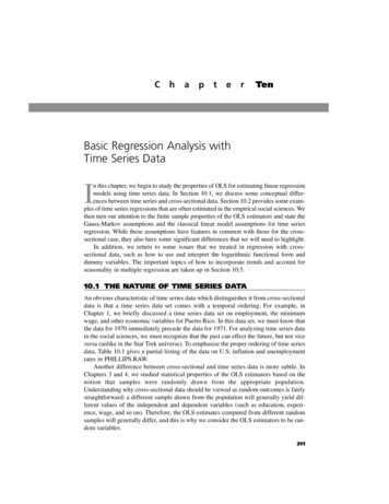
ram0.50Cross-correlations of gas and lninjuries1.00xcorr gas lninjuries, lags(10) xlabel(-10(1)10, grid)-10 -9 -8 -7 -6 -5 -4 -3 -2 -1 0 1Lag2 34 567 89 10There certainly appears to be at least some relationship between the price of gasoline and seriousvehicle crashes per month. However, there also appears to be consistent ‘bends and drops’ in thecross correlation, further evidence suggesting THE DATA ARE NOT STATIONARY!!Ideally, these would be very flat.16
xcorr gas lninjuries, lags(10) table. xcorr gas lninjuries, lags(10) xlabel(-10(1)10, grid). xcorr gas lninjuries, lags(10) 4-0.4658-0.4307.At lag 0, there is a -.297 correlation between fuel prices and serious crashes. Since the scale onthe IV is in dollars, a one dollar increase in fuel prices corresponds to a 29.7% IMMEDIATEreduction in the number of monthly serious vehicle crashes.However, the additional evidence of non-stationary series is seen given the lack of ‘flat spikes’.We need to test for stationarity.17
Let’s examine whether this series is stationary at immediate and specific points in time. One wayis to use the Augmented Dickey Fuller Test, which tests whether the series has a UNIT ROOT ( more than 1 trend in the series). It identifies if we have non-stationary data (at key lags).Remember, the Ho is that the series DOES have a unit root and a p .05 a unit root to dealwith (thus, p .05 NO UNIT ROOT, you can move on).dfuller lninjuries, lags (1). dfuller lninjuries, lags (1)Augmented Dickey-Fuller test for unit rootZ(t)TestStatistic1% CriticalValue-2.595-3.556Number of obs 67Interpolated Dickey-Fuller5% Critical10% CriticalValueValue-2.916-2.593MacKinnon approximate p-value for Z(t) 0.0941Test statistic (-2.595) and p value (.0941) indicate there IS A UNIT ROOT. This means theseries are not stationary at 1 lag.Let’s diagnose further at 2 lags.dfuller lninjuries, lags (2). dfuller lninjuries, lags (2)Augmented Dickey-Fuller test for unit rootZ(t)TestStatistic1% CriticalValue-2.674-3.558Number of obs 66Interpolated Dickey-Fuller5% Critical10% CriticalValueValue-2.917-2.594MacKinnon approximate p-value for Z(t) 0.0786.While an improvement (p-value went down to .078), it is still above our acceptable threshold,thus indicating both an immediate effect (t-1) and a secondary lagged effect (at t-2).In real life, you would have to stop here and find a better fit to make it acceptable. However, itcan’t be done with this outcome. That’s because it’s not a normally distributed outcome to beginwith. These results suggest that whatever model we identify, we control for immediate laggedeffects (plus any additional trends, such as seasonality, which we haven’t really tested for yet).18
Examine the Corrgramcorrgram lninjuries, lags(20)Why 20 lags now? Because at alpha .05, we would expect that BY CHANCE 1 out of every 20lags will have significant ‘noise’ – but no more than 1/20.The ACs correlation between the current value of the outcome (i.e., serious vehicle crashes)and the value of the outcome at time periods IMMEDIATELY before it. So, in the case below,the correlation between serious vehicle crashes and serious crashes 2 months prior .5809 (theyare smooth averaged). The AC is often used in model fitting when dealing with a stationaryseries and attempting to identify a MOVING AVERAGE (q) model.The PACs the correlation between the current value of serious vehicle crashes and its value atspecific points in time (WITHOUT THE EFFECT of the LAG BETWEEN T and T(lag)). So, inthis case, the correlation between serious vehicle crashes in a given month and 4 months ago .1385, without the effect of the 3 previous lags (between T and T(Lag of interest)). PACs can beused to define the autocorrelation in a stationary AR (p) series only.19
corrgram lninjuries, lags(20)If no parameters needed modeled, we’d see an exponential decay in the PACFs and possibly theACFs. We don’t see that here. We need to control for the underlying trend (notice also thePACFs go up a lot in the 12th month – indication of seasonality!).20
Plotting the ACF and PACF with confidence envelopes allows us to more closely see where thesignificant spikes occur (since we know we do not have a random walk process).ACF PLOTSac lninjuriesAutocorrelation functions indicate there is again no exponential decay to 0 – which is what wewould have if we had a random process. And, the spikes indicating autocorrelation appear quiteearly in the process. So, we need model out the immediate impact time has on the dependentvariable (i.e., when crashes are high, they’re also high in the previous/next period).21
PACF PLOTSpac lninjuriesPartial autocorrelation functions indicate ALTERNATING POSITIVE/NEGATIVE PACFS, aswell as spikes every 12 lags (potential seasonality).See the next page on the rules of thumb for model diagnosis.22
**Diagnosing the model and deciding which parameters to include (copied from 3Jenkins) – very consistent with most texts.ShapeExponential, decaying to zeroIndicated ModelAutoregressive model. Use the partial autocorrelation plot toidentify the order of the autoregressive model.Alternating positive and negative, Autoregressive model. Use the partial autocorrelation plot to helpdecaying to zeroidentify the order.One or more spikes, rest areessentially zeroDecay, starting after a few lagsAll zero or close to zeroHigh values at fixed intervalsNo decay to zeroMoving average model, order identified by where plot becomeszero.Mixed autoregressive and moving average (ARMA) model.Data are essentially random.Include seasonal autoregressive term.Series is not stationary.As you can see, diagnosing which parameters to include requires us to examine severalcomponents of each ARIMA model – since each time series is unique.My read on these data – it’s most likely either: A) AR1 12 month seasonal, or B) AR2 process 12 month seasonal (depending if that first lag drops when we control for seasonality).23
Let’s Compare Some Modelsarima lninjuries, ar(1, 12). arima lninjuries , ar(1, 12)(setting optimization to BHHH)Iteration 0: log likelihood Iteration 1: log likelihood Iteration 2: log likelihood Iteration 3: log likelihood Iteration 4: log likelihood (switching optimization to BFGS)Iteration 5: log likelihood Iteration 6: log likelihood Iteration 7: log likelihood Iteration 8: log likelihood 906448.33933948.33934648.339347ARIMA regressionSample: 2004m3 - 2009m11Number of obsWald chi2(2)Prob chi2Log likelihood 48.33935OPGStd. L1.L12.4677765.4346873/sigma.116545z 69126.490.0000P z [95% Conf. 0953210.640.000.0950772.1380128ARMANote: The test of the variance against zero is one sided, and the two-sided confidence interval is truncated at zero.Both autoregressive parameter estimates are statistically significant, indicating they fit the data.predict res1, rThis command also saves the residuals for this model.24[“, r” residuals.]
Graph the residuals for this initial ARIMA model.corrgram res1, lags(20)There is still evidence of significant autocorrelation at the early spikes. Specifically, lag 2 andlag 3 have p values .05. That is 2/20, and Lag 4 is marginally significant (p .08).I wouldn’t be comfortable moving forward modeling the intervention with this model becausethere is still some un-captured autocorrelation. Thus, including the intervention would lead to aninaccurate read of the potential intervention parameter.25
Let’s look at the AR2 12 month seasonalarima lninjuries, ar(2,12). arima lninjuries, ar(2,12)(setting optimization to BHHH)Iteration 0:log likelihood Iteration 1:log likelihood Iteration 2:log likelihood Iteration 3:log likelihood Iteration 4:log likelihood (switching optimization to BFGS)Iteration 5:log likelihood Iteration 6:log likelihood Iteration 7:log likelihood Iteration 8:log likelihood Iteration 9:log likelihood Iteration 10: log likelihood MA regressionSample:2004m3 - 2009m11Log likelihood Number of obsWald chi2(2)Prob chi247.01635OPGStd. rL2.L12.4308217.4634254/sigma.1181788z 69127.670.0000P z [95% Conf. 5.01384148.540.000.0910501.1453075ARMANote: The test of the variance against zero is one sided, and the two-sided confidence interval is truncated at zero.Again, both AR parameter estimates are statistically significant.Let’s examine the residuals.predict res2, r26
Now lets graph the residuals and examine the test statistics for noise parameters.corrgram res2, lags(20). predict res2, r. corrgram res2, 17.39421.5621.99823.208Prob Q-101 -101[Autocorrelation] [Partial 55170.42800.25210.28440.2787.Technically speaking (very technically), this model might be a suitable and acceptable fit. Ithonestly is the best fit I can model.Lag 1 is significant (lag 1, p .05, lag 2 is close, p .07, and no other spikes are significant).Due to chance alone, we expect 1/20 to be significant. This will pass the acceptability test. Inmy view, it doesn’t pass the ‘smell test’.Here is why - the fact the original outcome data aren’t normally distributed means we ‘waste’ anumber of transformations that we could use to address other time-variance issues.27
But, for the sake of moving on - we’ve identified a model without the intervention parameter thatfits our data without violating any major assumptions.The next step is to move to the analysis of the intervention. Again, we need to ‘wash away thesignificant underlying trend’ in the data in order to assess whether the intervention estimateinfluences our outcome above and beyond the trends we observe.The model is typed in as:arima lninjuries interven, ar(2,12). arima lninjuries interven , ar(2, 12)(setting optimization to BHHH)Iteration 0:log likelihood Iteration 1:log likelihood Iteration 2:log likelihood Iteration 3:log likelihood Iteration 4:log likelihood (switching optimization to BFGS)Iteration 5:log likelihood Iteration 6:log likelihood Iteration 7:log likelihood Iteration 8:log likelihood Iteration 9:log likelihood 1.56133351.56146651.56148351.561484ARIMA regressionSample:2004m3 - 2009m11Log likelihood Number of obsWald chi2(3)Prob chi251.56148OPGStd. Err.zP z 6944.260.0000lninjuriesCoef.[95% Conf. 8206ARMANote: The test of the variance against zero is one sided, and the two-sided confidence interval is truncated at zero.The AR parameters are still suitable (i.e., it’s okay that the L2 coefficient isn’t significant at .05– that sometimes happens when you add an intervention estimate to the model). The interventionestimate indicates that the logged number of serious vehicle crashes declined by -.182 (Exp(.182) -16.68%) in the post-intervention period relative to the pre-intervention period,controlling for serial autocorrelation at immediate as well as seasonal lags.28
An examination of the q-statistics from this model indicate the model is appropriate (at leasttechnically – in some ways, though again I wouldn’t be very comfortable with it, given thesignificant spike at lag 1).predict res3, rcorrgram res3, lags(20). corrgram res3, 32415.84916.46316.7820.09Prob Q-101 -101[Autocorrelation] [Partial 50100.53460.56030.60480.4523.Again, our examination of the residuals is less than ideal. If the model were a really good fit, wewould see no significant spikes at any of the first 20 lags.If there were to be a spike that would cause little concern (1/20, remember) – it would be later inthe series.29
Remember in t-tests, we estimated the decline in the monthly number of serious traffic crashes tobe roughly 21.2%?Well, when controlling for underlying trends in the series, the estimated effect was reduced toroughly -16.68%. This is almost always the case in all statistics!!! The more expected variationyou model, the less impact a specific estimate has on an outcome.When we do not control for underlying factors (i.e., the influence of some extraneous andimportant force) – we overstate our conclusions!Feel free to add the gas variable to the model just to add a time-varying control shown to predictchanges in vehicle crashes (to have a more theoretically accurate model).arima lninjuries interven gas, ar(2,12)ARIMA regressionSample:2004m3 - 2009m11Log likelihood Number of obsWald chi2(4)Prob chi251.62919OPGStd. 12.2096333.40296/sigma.112553z 6941.950.0000P z [95% Conf. 928.01281358.780.000.087439.1376671ARMANote: The test of the variance against zero is one sided, and the two-sidedconfidence interval is truncated at zero.While not a significant parameter itself – it does appear to reduce some of the magnitude of theintervention coefficient (to roughly 16.4%).If you have other time-varying measures to include that might explain changes in serious vehiclecrashes, this would be the time to incorporate them into the analysis and to add their results toyour table(s).30
Concluding Thoughts - ARIMAThis leads me to my next point. Which of these statistics should I present in my paper? Myanswer is that there is no ONE PERFECT analysis to display and write about.Although not an interrupted time series analysis per say – the Kovandzic et al. (2009) approach(Table 3, pp. 819-820) serves as a very good guide. I’ve followed this type of model in my ownresearch, keeping in mind interested readers are interested in the confidence interval around anestimate as well as whether or not an intervention estimate is statistically significant.3I find it best to show the reader of your paper how robust the intervention estimate is whenmodeling in different ways. The consistency and magnitude of an intervention estimate isprobably the most important dimension.Now, the ARIMA model used here was less than ideal. That is because in criminology andcriminal justice (in particular), we often model event count data.These data are notorious for being non-normalized. A widely used alternative approach tomodeling event count data with skewed outcomes is to rely on maximum likelihood estimation.That is what we will focus on next.3Kovandzic, T.V., Vieraitis, L.M., &
tsset date, monthly [designates time series, date variable in monthly format] *Delta the gap between measures (1 month)* Note: At the beginning of every time series analysis (i.e., every time you open a new time series file)– be sure to run the tsset command