WIXLIB

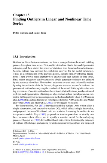
248P. Galeano, D. PeñaFig. 15.4 Stationary series with and without a LS15.2.1.4 Level ShiftsA level shift (LS) is a change in the mean level of the time series starting at t k andcontinuing until the end of the observed period. Therefore, a time series y1 , . . . , yTaffected by the presence of a LS at t k is given by:(k)yt xt wSt ,where St (1 B) 1 Itinnovations as follows:(k)(k)is a step function. Note that a LS serially affects the(k)at et π(B)wSt .Figure 15.4 shows a simulated series with sample size T 100 following anAR(1) model with parameter φ 0.8 and innovation variance σe2 1, joint withthe same series with a LS of size w 10 at t 50. Note how the LS affects all theobservation of the series after t 50. A LS has a strong effect in both identificationand estimation of the observed series. Indeed, the effect of an LS is close to theeffect of an IO on a nonstationary series.15.2.1.5 Temporary ChangesA temporary change (TC) is a change with effect that decreases exponentially.Therefore, a time series y1 , . . . , yT affected by the presence of a TC at t k isgiven by1(k)wI ,1 δB twhere δ is the exponential decay parameter such that 0 δ 1. Note that if δ tendsto 0, the TC reduces to an AO, whereas if δ tends to 1, the TC reduces to a LS.Under the presence of a TC, the innovations are affected as follows:yt xt at et π(B)(k)wI .1 δB t

15Finding Outliers in Linear and Nonlinear Time Series249Fig. 15.5 Stationary series with and without a TCThen, if π(B) is close to 1 δB, the effect of a TC on the innovations is very closeto the effect of an IO. Otherwise, the TC can affect several innovations.Figure 15.5 shows a simulated series with sample size T 100 following anAR(1) model with parameter φ 0.8 and innovation variance σe2 1, and the sameseries with an TC of size w 10 and decay rate δ 0.7 at t 50. Note how the TChave a decreasing effect in the observations of the series after t 50.15.2.1.6 Ramp ShiftsFinally, a ramp shift (RS) is a change in the trend of the time series in anARIMA(p, 1, q) model starting at t k and continuing until the end of the observed period. Therefore, a time series y1 , . . . , yT affected by the presence of a RSat t k is given by(k)yt xt wRt ,where Rt(k) (1 B) 1 St(k) is a ramp function. Note that a RS on the I (1) seriesyt is a LS on the differenced series (1 B)yt . Note also that a RS serially affectsthe innovations as follows:(k)at et π(B)wRt .Other types of unexpected events have been considered in the literature. For instance, variance changes have been considered in Tsay (1988), while patches ofadditive outliers have been studied in Justel et al. (2001) and Penzer (2007). Modeling alternative unexpected events is also possible as the intervention framework isflexible enough to model many different situations. For example, new effects can bedefined using combinations of the outliers previously considered.

250P. Galeano, D. Peña15.2.2 Outlier Identification and EstimationIn general, all the types of outliers that we have presented can be written in a generalequation:(k)yt xt ν(B)wIt ,(15.3)where ν(B) 1 for an AO, ν(B) ψ(B) for an IO, ν(B) (1 B) 1 for a LS,ν(B) (1 δB) 1 for a TC and ν(B) (1 B) 2 for a RS, respectively. Therefore, outliers in time series can be seen as particular cases of interventions, introduced by Box and Tiao (1975), to model dynamic changes on a time series at knowntime points.Assume that we observe a series, y1 , . . . , yT , following an ARIMA(p, d, q)model as in (15.1) with known parameters and with an outlier of known type att k. Multiplying by π(B) in (15.3) leads to the equation for the innovations:at et wi zi,t ,(15.4)for i AO, IO, LS and TC, where wAO , wIO , wLS and wTC is the size of the outlier(k)for AO, IO, LS and TC, respectively, and zi,t π(B)νi (B)It , where νAO (B) 1, 1νIO (B) ψ(B), νLS (B) (1 B) and νTC (B) (1 δB) 1 , respectively. From(15.4), for any particular case, one can easily estimate the size of the outlier by leastsquares leading to: Tzi,t atŵi t 1T2t 1 zi,t 2 ) 1 . Consequently, knowing the type andwith variance ρi2 σe2 where ρi2 ( Tt 1 zi,tlocation of the outlier, it is easy to adjust the outlier effect on the observed seriesusing the corresponding estimates, ŵAO , ŵIO , ŵLS or ŵTC , respectively.Also, the estimates of the outlier size can now be used to test whether one outlierof known type has occurred at t k. Indeed, the likelihood ratio test statistic for thenull hypothesis H0 : wi 0 against the alternative H1 : wi 0, is given byτi,k ŵi,k.ρi σeThe statistic τi,k , under the null hypothesis, follows a Gaussian distribution.However, in practice, the number, location, type and size of the outliers are unknown. Several papers, including Chang et al. (1988), Tsay (1988), Chen and Liu(1993a) and Sánchez and Peña (2010), among others, have proposed iterative procedures in which the idea is to compute the likelihood ratio test statistics for all theobservations of the series under the null hypothesis of no outliers. In particular, theprocedure by Chen and Liu (1993a), which is standard nowadays, works as follows.In a first step, an ARIMA model is identified for the series and the parameters are estimated using maximum likelihood. Then, the likelihood ratio test statistics τi,t , for

15Finding Outliers in Linear and Nonlinear Time Series251i AO, IO, LS and TC, are computed. If the maximum of all these statistics is significant, an outlier of the type that provides with the maximum statistic is detected.Then, the series is cleaned of the outlier effects and the parameters of the modelare re-estimated. This step is repeated until no more outliers are found. In a secondstep, the outliers effects and the ARIMA model parameters are estimated jointlyusing a multiple regression model. If some outlier is not significant, it is removedfrom the outliers set. Then, the multiple regression model is re-estimated. This stepis repeated until all the outlier effects are significant. In a final step, the two previous steps are repeated but initially using the ARIMA model parameters estimatesobtained at the end of the second step. However, this procedure has three main drawbacks. First, when a level shift is present in the series, the procedure tends to identifyan innovative outlier instead of the level shift. Second, the initial estimation of themodel parameters usually leads to a very biased set of parameters that may producethe procedure to fail. Third, the masking and swamping effects, although mitigatedwith respect to previous procedures, are still present if a sequence of outlier patchesis present in the time series. Sánchez and Peña (2010) proposed a procedure for multiple outlier detection and robust estimation that tries to avoid these three problems.In particular, to solve the first problem, it is proposed to compare AO versus IO anddeal with LS alone. To solve the second problem, it is proposed to use influencemeasures to identify the observations that have a larger impact on estimation andestimate the parameters assuming that the most influential observations are missing.Finally, to solve the third problem, an influence measure for LS or sequences ofpatchy outliers is proposed that can be used to carry out the initial cleaning of thetime series.15.3 Outliers in Nonlinear Time Series ModelsThis section reviews outliers in some nonlinear time series models. In particular, wefirst consider the model-based method proposed by Battaglia and Orfei (2005) fordetecting the presence of outliers when the series is generated by a general nonlinearmodel. Second, we summarize the effect of outliers in GARCH models followingCarnero et al. (2007) and present a method proposed by Hotta and Tsay (2012) fordetecting outliers in GARCH models. Finally, we describe the method proposed byFokianos and Fried (2010) to detect outliers in INGARCH models.15.3.1 Outliers in a General Nonlinear ModelBattaglia and Orfei (2005) assumed a time series xt following the model: xt f x(t 1) , e(t 1) et ,(15.5)

252P. Galeano, D. Peñawhere f is a nonlinear function also containing unknown parameters, x(t 1) (xt 1 , xt 2 , . . . , xt p ) , e(t 1) (et 1 , et 2 , . . . , et p ) and et is a white noise sequence of independent and identically distributed (i.i.d.) Gaussian with mean zeroand variance σe2 . Note that the model in (15.5) covers several well known nonlinear models, such as the bilinear model, the self-exciting threshold autoregressive(SETAR) model and the exponential autoregressive model, among others.For the model in (15.5), Battaglia and Orfei (2005) consider additive and innovative outliers. First, for an AO at t k, the observed series is y1 , . . . , yT ,given by yt xt wIt(k) , for t 1, . . . , T , where xt follows the model in (15.5).Therefore, the observed series can be written as yt f (y(t 1) , a(t 1) ) at , wherey(t 1) (yt 1 , yt 2 , . . . , yt p ) and a(t 1) (at 1 , at 2 , . . . , at p ) , respectively,for t 1, . . . , T . The innovations of the observed series can be obtained recursivelyfrom at yt f (y(t 1) , a(t 1) ). On the other hand, for an IO at t k, the ob(k)served series is given by yt f (y(t 1) , a(t 1) ) at , where at et wIt , wherey(t 1) (yt 1 , yt 2 , . . . , yt p ) and a(t 1) (at 1 , at 2 , . . . , at p ) , respectively,for t 1, . . . , T .Estimation of outlier effects can be done similarly to the ARIMA case throughleast squares. Battaglia and Orfei (2005) showed that the LS estimate of w for anIO is given by ŵIO ak with variance σe2 , and that the LS estimate of w for an AOis given by T kj 0 cj ak jŵAO T k2j 0 cj k 2 2with variance ( jT 0cj )σe , where cj f y (k j 1) , a (k j 1) yt jji 1 (k j 1) (k j 1) cj if y,a, at jfor j 1, . . . , T k. Consequently, the likelihood ratio test statistics to test for thepresence of an AO and a IO at t k are given byτIO andak,σe T kj 0 cj ak jτAO ' ,T k 2j 0 cj σerespectively. Under the null hypothesis of no outlier, τAO and τIO have a standardGaussian distribution.In order to detect the presence of several outliers in a nonlinear time series,Battaglia and Orfei (2005) considered a procedure similar to that used in Chen andLiu (1993a).

15Finding Outliers in Linear and Nonlinear Time Series25315.3.2 Outliers in GARCH ModelsCarnero et al. (2007) have analyzed the effects of outliers on the identification andestimation of GARCH models. Regarding identification, Carnero et al. (2007) derived the asymptotic biases caused by outliers on the sample autocorrelations ofsquared observations generated by stationary processes and obtained the asymptoticbiases of the ordinary least squares (OLS) estimator of the parameters of ARCH(p)models. Finally, these authors also studied the effects of outliers on the estimatedasymptotic standard deviations of the estimators considered and showed that theyare biased estimates of the sample standard deviations.Recently, Hotta and Tsay (2012) have distinguished two types of outliers inGARCH models and have proposed a method for their detection. For simplicityof presentation, we consider the ARCH(1) model given byxt ht et ,2ht α0 α1 xt 1,where α0 0, 0 α1 1, and et are independent and identically distributed standard Gaussian random variables. Outliers in an ARCH(1) model encounter two different scenarios because an outlier can affect the level of xt or the volatility ht .Therefore, a volatility outlier, denoted by VO, and defined as followsyt ht et wIt(k) ,2ht α0 α1 yt 1affects the volatility of the series, while a level outlier, denoted by LO, and given by(k)yt ht et wIt , (k) 2ht α0 α1 yt 1 wIt 1only affects the level of the series at the observation where it occurs.Hotta and Tsay (2012) estimated w by means of the ML estimation method.These authors showed that the ML estimate of w for a VO is given byŵVO yk ,and that there are two ML estimates of w for a LO: the first one is ŵLO yk and thesecond one is ŵLO yk x̂k , where x̂k is the square root of the positive solutionof the second order equation: 2xg(x) α12 x 2 2α0 α1 α12 α0 α1 yk 1 2222 α1 yk 1α0 α1 yk 1, α0 α0 α1 α0 α1 yk 1provided that such a solution exists.

254P. Galeano, D. PeñaIn order to test for the presence of a VO or a LO, Hotta and Tsay (2012) proposethe use of the Lagrange multiplier (LM) test statistic that, for a VO, is defined asyk2LMVOk 2α0 α1 yk 1,while for a LO, it is given by 2 2 yk 1yk2 11VO2LMLO1 α1 2α LMh h.1 k1 k 2kkhk 1 h2k 1hk 1VONote that LMLOk LMk if α1 0. Therefore, the two test statistics should notdiffer substantially when α1 is close to 0. To detect multiple outliers, Hotta andTsay (2012) thus propose to compute the maximum LM statisticsVOLMVOmax max LMk ,2 t nLOLMLOmax max LMk ,2 t nfor which it is easy to compute critical values via simulation. If both statistics aresignificant, one may choose the outlier that gives the smaller p-value.15.3.3 Outliers in INGARCH ModelsFokianos and Fried (2010) consider outliers in the integer-valued GARCH (INGARCH) model given byxxt Ft 1 Poisson(λt ),pλt α0 qαj λt j j 1(15.6)βi xt i ,i 1xstands for thefor t 1, where λt is the Poisson intensity of the process xt , Ft 1σ -algebra generated by {xt 1 , . . . , x1 q , λt 1 , . . . , λ0 }, α0 is an intercept, αj 0, p qfor j 1, . . . , p and βi 0, for i 1, . . . , q and j 1 αj i 1 βi 1 to getcovariance stationarity. Outliers in the INGARCH model (15.6) can be written asyyt Ft 1 Poisson(κt ),pκt α0 qβi yt i w(1 δB) 1 It ,(k)αj κt j j 1(15.7)i 1yfor t 1, where κt is the Poisson intensity of the process yt , Ft 1 stands for theσ -algebra generated by {yt 1 , . . . , y1 q , κt 1 , . . . , κ0 }, w is the size of the outlier,

15Finding Outliers in Linear and Nonlinear Time Series255and 0 δ 1 is a parameter that controls the outlier effect. In particular, δ 0 corresponds to an spiky outlier (SO) that influences the process from time k on, but to arapidly decaying extent provided that α1 is not close to unity, 0 δ 1 correspondsto a transient shift (TS) that affects several consecutive observations although its effect becomes gradually smaller as time grows and, finally, δ 1 corresponds to alevel shift (LS) that affects permanently the mean and the variance of the observedseries.Fokianos and Fried (2010) propose to estimate the outlier effect w via conditionalmaximum likelihood. Therefore, given the observed time series y1 , . . . , yT , the loglikelihood of the parameters of model (15.7), η (α0 , α1 , . . . , αp , β1 , . . . , βq , w) yconditional on F0 is given, up to a constant, byT7 yt log κt (η) κt (η)!(η) (15.8)t q 1with score function l(η) η Tt q 1 yt κt (η) 1.κt (η) ηIn addition, the conditional information matrix for η is given byTG(η) t q 1 l(η) yCov Ft 1 ηTt 1 l(η) l(η) 1.κt (η) η ηConsequently, ŵ is obtained from the ML estimate η̂ after maximizing the loglikelihood function (15.8). In order to test for the presence of an outlier at t k,Fokianos and Fried (2010) propose to use the score test given byTk G(α̃0 , α̃1 , . . . , α̃p , β̃1 , . . . , β̃q , 0) 1 ,where l(α̃0 , α̃1 , . . . , α̃p , β̃1 , . . . , β̃q , 0), ηand (α̃0 , α̃1 , . . . , α̃p , β̃1 , . . . , β̃q , 0) is the vector that contains the ML estimates ofthe parameters of the model (15.6) and the value w 0. Under the null hypothesisof no outlier, Tk has an asymptotic χ12 distribution. To detect an outlier of a certaintype at an unknown time point, the idea is to obtainT max Tt ,q 1 t Tand reject the null hypothesis of no outlier if T is large. The distribution of thisstatistic can be calibrated using bootstrap. Finally, to detect the presence of severaloutliers in a INGARCH time series, Fokianos and Fried (2010) proposed a procedure similar to that used in Chen and Liu (1993a).

256P. Galeano, D. Peña15.4 Outliers in Multivariate Time Series ModelsOutliers in multivariate time series has been much less analyzed than in the univariate case. Multivariate outliers were introduced in Tsay et al. (2000). These authorshave also proposed a detection method based on individual and joint likelihood ratio statistics. Alternatively, Galeano et al. (2006) used projection pursuit methodsto develop a procedure for detecting outliers. In particular, Galeano et al. (2006)showed that testing for outliers in certain projection directions can be more powerful than testing the multivariate series directly. In view of these findings, an iterativeprocedure to detect and handle multiple outliers based on a univariate search inthese optimal directions were proposed. The main advantage of this procedure isthat it can identify outliers without prespecifying a vector ARMA model for thedata. An alternative method based on linear combinations of the components of thevector of time series can be found in Baragona and Battaglia (2007b) that considersan independent component approach. Finally, Baragona and Battaglia (2007a) haveproposed a method to discover outliers in a dynamic factor model based on lineartransforms of the observed time series. In this section, we briefly review the mainfindings in Tsay et al. (2000) and Galeano et al. (2006).15.4.1 The Tsay, Peña and Pankratz ProcedureA r-dimensional vector time series Xt (X1t , . . . , Xrt ) follows a vector ARMA(VARMA) model ifΦ(B)Xt C Θ(B)Et ,t 1, . . . , T ,(15.9)where Φ(B) I Φ1 B · · · Φp B p and Θ(B) I Θ1 B · · · Θq B q arer r matrix polynomials of finite degrees p and q, C is a r-dimensional constant vector, and Et (E1t , . . . , Ert ) is a sequence of independent and identically distributed Gaussian random vectors with zero mean and positive-definitecovariance matrix Σ . The autoregressive representation of the VARMA modelin (15.9) is given by Π(B)Xt CΠ Et , where Φ(1)CΠ C and Π(B) iΘ(B) 1 Φ(B) I i 1 Πi B , while the moving-average representation of Xt isgiven by Xt CΨ Ψ (B)Et , where Φ(1)CΨ C and Φ(B)Ψ (B) Θ(B) with iΨ (B) I i 1 Ψi B .Tsay et al. (2000) generalize four types of univariate outliers to the vectorcase. Under the presence of a multivariate outlier, we observe a time series Y (Y1 , . . .

15 Finding Outliers in Linear and Nonlinear Time Series 247 Fig. 15.2 Stationary series with and without an IO Fig. 15.3 Nonstationary series with and without an IO effects due to internal causes. The innovations of a time series y1,.,yT affected by the presence of an IO at time point t kis given by: a t et wI (k), (15.2) where et are the innovations of the clean series xt.