Transcription
Beginning Steps in SPSSKeith E. EmmertSoad EmmertDepartment of Mathematics, Tarleton State UniversityE-mail address: emmert@tarleton.eduDepartment of Mathematics, Tarleton State UniversityE-mail address: semmert@tarleton.edu
ContentsChapter 1. First Steps with SPSS1.1. Introduction1.2. Entering Data1.3. Opening an Existing Dataset1.4. Changing How Variables are Listed1.5. Analyzing a Dataset1.6. Creating a Box plot1.7. Creating Histograms and Q-Q Plots1.8. Standardized Scores z-Scores1.9. Scatter Plots and Regression1.10. Testing Hypotheses about Population Means Using the t-Distribution1.11. χ2 Goodness of Fit1.12. Contingency Tables or Cross Tabulations – Testing for Independence1.13. Two-Sample Inference1.14. One-Way ANOVAv1112345914141618202327
CHAPTER 1First Steps with SPSS1.1. IntroductionSPSS stands for Statistical Package for the Social Sciences. It was developed in 1968, by NormanH. Nie, C. Hadlai (Tex) Hull and Dale H. Bent. Norman, frustrated with mainframe software which wasinadequate for his needs, needed a program to quickly analyze volumes of social science data gatheredthrough various methods of research. They wrote SPSS, the first of its kind, and targeted the PC. Theybegan selling to other professors at other universities and by 1974 was making over 200,000 per year –without marketing!1.2. Entering DataWhen you first open SPSS, you will see a window asking you what you would like to do in SPSS,much like that in Figure 1. To start creating your own dataset, select the “Type in data” option.Figure 1. Splash Screen for SPSSOnce you click the “OK” button, you will be given a blank data table. Now, click on the VariableView tab located at the bottom left corner of the window. Here is where you will declare your variables.You will notice that the column headers have changed. The column headers should look like the headersin Figure 2Figure 2. Variables Tab for SPSS1
21. FIRST STEPS WITH SPSSFor the purposes of this tutorial, we will create a simple dataset with two variables. The datasetwill contain a list of people’s height and gender.To start entering your variables, type the name of the variable into the “Name” box. The defaultvalues are loaded into all the other boxes. To change the variable type, click the grey dotted area inthe ”Type” box. The window shown in Figure 3 should open. This is where you can select the variabletype. For our example we leave “Height” as a numeric and change the default value of “Gender” to bea string.Figure 3. Entering Variables in SPSSNow that we have declared our variables, we can start entering the data. To add the data, click onthe Data View tab located at the bottom left corner. The following window will appear, where youcan add the data. The window will look as shown in Figure 4Figure 4. Entering Data in SPSS using the Data ViewTo save the given dataset, click on the File menu and choose Save. The following window willappear. Here you can choose the location of where you want to save the dataset. By default your file issaved in a “.sav” format.1.3. Opening an Existing DatasetTo open a dataset, open SPSS and the following screen will appear as shown in Figure 5. Choose”Open an existing data source.”The textbook contains many datasets which are located on the CD. By default, the only datasetsthat will be visible will be datasets that have the file extension “.sav.” However, many of the olderdatasets will have the “.sys” extension. To view these, just change the “Files of types:” drop-downmenu setting to “SYS/PC ” and you will be able to see the .sys files.
1.4. CHANGING HOW VARIABLES ARE LISTED3Figure 5. Open a Saved Data Set in SPSS1.4. Changing How Variables are ListedWhen you start to run analyses, you will find that the variables will be listed by their label inthe order they appear on the dataset. Because some datasets can contain over 100 variables, finding aspecific variable can be difficult. You can change the way the variables are listed by using the Optionswindow. This can be reached by choosing Options under the Edit menu. Here we can change thedisplay to list the data sets in alphabetical order (instead of file) and to display the “Names” instead ofthe “Labels.” After choosing your options, click “OK,” as can be ssen in Figure 6. A warning about thechanging of options in the Variable List group will reset all dialog box setting will be displayed. Justclick “OK.” Now, when you run an analysis, the variables will be listed by their name in alphabeticalorder. This greatly speeds up the process of finding variables.Figure 6. Options Window in SPSS. Change to alphabetical listing of variables anddisplay names.
41. FIRST STEPS WITH SPSS1.5. Analyzing a DatasetThis is where we begin to perform statistics. Click on the Analyze menu. We will be using theFrequencies analysis, so go to the Descriptive Statistics sub-menu and select Frequencies., asshown in Figure 7.Figure 7. Select to perform descriptive statistics using the Frequencies. option.The Frequencies. option allows you to analyze variables individually as opposed to analyzingthem in relation with another variable. With this type of analysis, you can measure a variable’s individualproperties such as mean, median, mode, etc.To start the analysis, in the Frequencies window, move the variables you wish to analyze fromthe left list to the right list. This is done by selecting the variables from the left list and clicking theright-arrow button located between the two lists. If you wish to remove a variable, simply reverse theprocess and move it back to the left list. See Figure 8.Figure 8. The Frequencies. dialog window.Once you have chosen the required variables and set your display options, click the “OK” button.Another window will open up with the outputs displayed in the following format as shown in Figure 9.You can save this output window by clicking on the “Save” button. You can close this window oncethe output has been saved. You can also delete the output, by clicking on the “Output” option in the leftwindow, and then hitting the “Delete” button. If you leave this window open, and run another analysis,then the output for that run will be stacked under the existing output. If you print this output, then
1.6. CREATING A BOX alid tal6100.0100.0Figure 9. The Frequencies. results.all the analysis outputs will be printed, so it is recommended that you delete the output analysis fromthe output window once you have saved them.For the rest of this section, you will need to change how the variables are listed in the analysiswindows. If you need help, please refer to Section Four: Changing how variables are listed.If you wish to see some basic descriptive statistics, then choose Analyze followed by Descriptive Statistics followed by Frequencies. Again, you select your variable (Height) and choose theStatistics. button as shown in Figure 10.Figure 10. The Frequencies. dialog - accessing the Statistics.options.This will open a new window, the Frequencies: Statistics dialog box. Check Mean, Median,Mode, Variance, Standard Deviation, Range, and Quartiles. Press the “Continue” button.Now choose “OK.” SPSS should stack the results below your frequencies as seen in Figure 12. Noticethat SPSS calculates the five number summary, plus x̄, s, s2 , and range.1.6. Creating a Box plotPage 1Let’s open up a larger data set. SPSS provides us with “cars.sav.” There are several variables in the“cars.sav” data set: mpg, engine, horse, weight, accel (0 - 60 mph), year (1970 - 1982), origin, cylinder,and filter .First, let’ create a boxplot for mpg. Choose Analyze - Descriptive Statistics - Explore. toopen the Explore dialog box as shown in Figure 13. Go ahead and add “mpg” to the Dependent Listand select “Plots” i the Display group.Next, select the Plots. button which opens the Explore:Plots dialog box, as can be seen inFigure 14. Select “Factor levels together” (it should already be selected) in the “Boxplots” group anduncheck “Stem-and-leaf” in the “Descriptive” group.Select Continue and then OK. The results will appear in an output window and should look likethe image in Figure 15. Notice that one outlier (observation #330) is plotted as a circle.
61. FIRST STEPS WITH SPSSFigure 11. The Frequencies: Statistics dialog - accessing the additional ng0Mean69.1667Median68.5000Mode66.00Std. 0Figure 12. The Descriptives. results: Five number summary, plus x̄, s, s2 , and range.Figure 13. The Explore. dialog for exploring data sets.
1.6. CREATING A BOX PLOT7Figure 14. The Explore:Plots. dialog for exploring data sets.50330403020100Miles per GallonFigure 15. The box plot for mpg.Of course, this is a bit misleading since it combines cars over a span of 13 years. Perhaps we shouldbreak them up into smaller pieces.To make box plots for the mpg based upon a given year, choose Analyze - Descriptive Statistics- Explore. to open the Explore dialog box as shown in Figure 16. Notice that I have already added“mpg” to the Dependent List, “year” to the Factor List, and selected “Plots” in the Display group.Click the Plots. button to open the Explore: Plots dialog box as shown in Figure 17. Choose thebullet for “Factor levels together” to make a separate Boxplot for each of the variables in the “DependentList” in the Explore dialog box. If there are several variables in the Dependent List, choose the bulletfor Dependents together to obtain side-by-side Boxplots.Select Continue and then OK. The resulting side-by-side box plots are shown in Figure 18.Page 1
81. FIRST STEPS WITH SPSSFigure 16. The Explore. dialog for exploring data sets.Figure 17. The Explore:Plots. dialog for exploring data sets.50252Miles per Gallon4030201070717273747576777879808182Model Year (modulo 100)Figure 18. The side-by-side box plots of mpg based upon a given year.Page 1
1.7. CREATING HISTOGRAMS AND Q-Q PLOTS9Suppose that you wish to view side-by-side box plots of mpg and acceleration based upon year. Theprocedure is virtually the same. Just add the “Accel” variable to the “Dependent List” and click onthe Plots. button to open the Explore:Plots dialog. In the Explore:Plots dialog, make sure youselect “Dependents together” in the “Boxplots” section. The resulting side-by-side boxplots are shownin Figure 19.Miles per GallonTime to Accelerate from 0to 60 mph 879808182Model Year (modulo 100)Figure 19. The side-by-side box plots of mpg and acceleration based upon a given year.It is interesting to notice that during certain years, ’72, ’74, ’78, ’79, and ’82, there are instances ofcars that have extremely slow acceleration. In ’78, there is a car that received exceptional gas mileage.Notice that this was not the slowest car that year, either (but if you look at the data set, it was close).1.7. Creating Histograms and Q-Q PlotsLet’s first see what how a histogram and Q-Q plot from a normal distribution looks like. The plotsin Figure 20 were generated from 200 samples of a random variable which follows N ((2, 1.26492 ).Notice that in Figure 20a, we see a histogram. It is unimodal (mound shaped) and symmetric, bothof which are characteristics of a normal distribution. Now, in Figure 20b, we see a Q-Q Plot. Most ofthe sample are grouped in the middle (again indicating symmetry). More importantly, most of the data(i.e. in the middle) lies on a straight line. The straight line is a “perfect” normal distribution (usingPage 1 to this line, thethe sample mean and standard deviation, that is N (2.09, 1.2392 )), so the closer we comemore likely we have stumbled across a normal distribution.Now, let’s compare some non-normal histograms and Q-Q plots. We’ll consider samples from abinomial random variable, binomial(10, 0.2), log-normal with parameters 2 and 0.5, and finally a uniformwith parameters 1.8 and 5.8.First, the binomial random variable. Figures 21a and 21b are the histogram and Q-Q Plot for thisbinomial random variable. Notice that the mean is µ 2 and the standard is σ 1.2649, which is the
101. FIRST STEPS WITH SPSSHistogramNormal Q-Q Plot of normal40Mean 2.09Std. Dev. 1.239N 2002Expected 2normal0246Observed Value(a) Histogram for a Normal Random Variable(b) Q-Q Plot for a Normal Random VariableFigure 20. Histogram and QQ-Plot for a Normal Random Variable.same as the mean and standard deviation of the normal used above. Notice that the histogram showsthat the binomial is a bit right skewed and certainly not very symmetric. The Q-Q Plot only lists pointson integer values (duh!, it’s a binomial! It counts successes). Clearly, this is not a normal distribution.Page 1Page 1HistogramNormal Q-Q Plot of binomial603Mean 2.16Std. Dev. 1.299N 20050Expected 5.000binomial246Observed Value(a) Histogram for a Binomial Random Variable(b) Q-Q Plot for a Binomial Random VariableFigure 21. Histogram and QQ-Plot for a Binomial Random Variable.Next, the log-normal random variable, which is a continuous random variable. Figures 22a and 22bare the histogram and Q-Q Plot for this log-normal random variable. Notice that the histogram showsthat the log-normal is a definitely right skewed and not symmetric. In the Q-Q PLot, data is groupedclosely together, just not the middle 50% portion of the data. Also, on the ends of the Q-Q Plot, thedata moves significantly away from the line. This indicates potential outliers and is not usual for anormal random variable. Again, this is not a normal distribution.Page 1Page 1
1.7. CREATING HISTOGRAMS AND Q-Q PLOTSHistogram11Normal Q-Q Plot of lognormal306Mean 2.36Std. Dev. 1.102N 200Expected 07.00024lognormal68Observed Value(a) Histogram for a Log-Normal Random Variable(b) Q-Q Plot for a Log-Normal Random VariableFigure 22. Histogram and QQ-Plot for a Log-Normal Random Variable.Finally, we consider a uniform random variable, which is a continuous random variable. Figures 23aand 23b are the histogram and Q-Q Plot for this uniform random variable. Notice that the histogramshows that the uniform is a definitely right skewed and not symmetric. In the Q-Q PLot, data is groupedclosely together, just not the middle 50% portion of the data. Also, on the ends of the Q-Q Plot, thedata moves significantly away from the line. This indicates potential outliers and is not usual for anormal random variable. Again, this is not a normal distribution.Page 1Page 1HistogramNormal Q-Q Plot of uniform203Mean 1.78Std. Dev. 2.172N 2002Expected 2.5uniform0.02.55.07.5Observed Value(a) Histogram for a Uniform Random Variable(b) Q-Q Plot for a Uniform Random VariableFigure 23. Histogram and QQ-Plot for a Uniform Random Variable.One final check is using one of the tests of normality. SPSS uses Kolmogorov-Smirnov and ShapiroWilk. Note that Shapiro-Wilk only applies to sample sizes up to 2,000. There are other tests that arePage 1Page 1
121. FIRST STEPS WITH SPSSmore useful in other situations. It is quite dangerous to use these tests on small sample sizes, especially 10. The Kolmogorov-Smirnov test may have some problems with large sample sizes, say 1, 000. Inall cases, the particular hypotheses being tested areH0 : The data is from a normal distribution.Ha : The data is NOT from a normal distribution.A failure to reject indicates that the sample appears to come from a normal distribution.See Figure 24. For the sample coming from a normal distribution, the Sig. is 0.200 for KolmogorovSmirnov and 0.411 for Shapiro-WIlk. Hence, we fail to reject H0 . It appears that the sample (basedupon this test) comes from a normal distribution. Compare this to binomial, lognormal, and uniform.All have small p-values, certainly less that 0.05. Hence, the conclusion is that the sample does not appearto be from a normal distribution.Tests of 0.411uniform.068200.956200.000.200*.025a. Lilliefors Significance Correction*. This is a lower bound of the true significance.Figure 24. Summary of Tests of NormalityFirst, you need to open a data file to analyze. We will analyze “EmployeeData.sav.” SelectAnalyze Descriptive Statistics Explore. Select the variable “Salary” and add it to the “DependentList.” Click on “Plots.” and select “Histogram” and “Normality plots with tests.” Deselect the “Stemand-leaf” box. See Figure 25. Click “Continue” and “OK” to run the procedure. You should obtainFigure 25. Explore:Plots, used to create Histograms and Q-Q PlotsPage 1output as seen in Figure 26.
1.7. CREATING HISTOGRAMS AND Q-Q PLOTS13The histogram and Q-Q Plot are shown in Figures 26a and 26b. Notice that most of the data isconcentrated to the left. This is clearly seen in the histogram. The Q-Q Plot also has a distinct bend init. These characteristics suggest that the data is not normally distributed.HistogramNormal Q-Q Plot of Current Salary120Mean 34,419.57Std. Dev. 17,075.661N 4747.5100Expected Normal5.0Frequency80602.50.040-2.5200 25,000 50,000 75,000 100,000 125,000025,00050,000Current Salary75,000100,000125,000Observed Value(a) Histogram for Salary(b) Q-Q Plot for SalaryFigure 26. Histogram and QQ-Plot for Salary.Another simple visual check is to overlay a normal curve using the calculated sample mean andsample standard deviation on top of your histogram. If the data is normally distributed, then theyshould (mostly) agree. In the histogram shown in Figure 28a, a normal curve in also plotted with thesame mean and standard deviation as the data. Notice that this does not match up well with thehistogram. Compare this to the data which was taken from a normal distribution (i.e. N (2.1, 1.26492 )at the beginning of this section; see also Figure 20a, the histogram without the normal curve). Thehistogram with a superimposed normal curve shown in Figure 28b has a much closer fit.In order to superimpose a normal curve onto a histogram, open your data set, such as “EmployeeData.sav.” Select Analyze Descriptive Statistics Frequencies. Then, select the variable, such as“Salary” and click the “Charts” button. Select the “Histograms” radio button and then click the “Shownormal curve on histogram” box. See Figure 27.Page 1Figure 27. Frequences: Charts - Creating Histograms with Normal CurvesPage 1
141. FIRST STEPS WITH SPSSHistogramHistogram12040Mean 34,419.57Std. Dev. 17,075.661N 474Mean 2.09Std. Dev. 1.239N 20010030FrequencyFrequency80602040102000 0 25,000 50,000 75,000 100,000 125,000-4.00-2.00.00Current Salary2.004.006.00normal(a) Histogram with Normal Curve for Salary(b) Histogram with Normal Curve using Normal DataFigure 28. Histogram and Normal Curves.Finally, in Figure 29, we see the statistical tests for normality. The extremely low significance levelof 0.0000 indicates a very strong rejection of H0 . That is, we are fairly confident that the data does notcome from a normally distributed population.Page 1Page 1Tests of NormalityKolmogorov-SmirnovStatisticCurrent Sig.474.000a. Lilliefors Significance CorrectionFigure 29. Summary of Tests of Normality for Salary.1.8. Standardized Scores z-ScoresCreating standardized scores is quick and painless using SPSS. Open any data file, such as “EmployeeData.sav.” Select Analyze Descriptive Statistics Descriptives. Select a variable of interest, such as“Salary” and click the “Save Standardized Values as Variables” box, as shown in Figure 30. A newcolumn of data will be created for each selected variable.1.9. Scatter Plots and RegressionOne of the first things you should do with a new data set is to look at it pictorially. If youhave response and explanatory variables, then one simple graph is a scatter plot. Open the data set“customer subset.sav”. Using SPSS, select Graphs Legacy Dialogs Scatter/Dot. Select the “SimpleScatter” option in the Scatter/Dot dialog box and click “Define”. For the y-axis, use the variable“carvalue” and for the x-axis use the variable “income”. Click “OK“. The results can be found inFigure 31.Notice that there does appear to be a linear trend in the data. So, perhaps we should perform linearregression. Linear regression is quickly performed by selecting Analyze Regression Linear. This opensPage 1
1.9. SCATTER PLOTS AND REGRESSION15Figure 30. Saving Selected Variables as z-Scores.100.00Primary vehicle sticker 0.00250.00300.00Household income in thousandsFigure 31. Scatter Plot of Primary Vehicle Sticker Price vs Household Income in Dollars.the Linear Regression dialog box. Select “carvalue” for the Dependent (y-variable) and “income” forthe Independent (x-variable). Clicking “OK” performs the requested regression. A lot of output isgenerated, but the more interesting part is shown in Figure 32. Notice that the significance level for theslope is 0.000 (which really means that it is really small.i.e. 0.001 but probably not zero). Thus wereject the null hypothesis that the slope of the regression line is zero and conclude that linear regressiondoes appear to be appropriate for our situation. The regression line is given byPage 1ŷ 0.401x 4.310so an increase of 1,000 dollars in household income increases the sticker price by 0.401 thousands, thatis 401.Another useful bit of information is the R value, Pearson’s Correlation Coefficient. Based on theinformation shown in Figure 33, we see that R 0.925, which indicates a strong, positive, linearassociation between the two variables.
161. FIRST STEPS WITH SPSSCoefficientsaUnstandardized CoefficientsBModel1(Constant)Household income inthousandsStandardizedCoefficientsStd. 9.000a. Dependent Variable: Primary vehicle sticker priceFigure 32. Linear Regression of Primary Vehicle Sticker Price vs Household Incomein Dollars.Model SummaryModel1RR Squarea.925.856Adjusted RSquare.854Std. Error ofthe Estimate8.07692a. Predictors: (Constant), Household income in thousandsFigure 33. R from Linear Regression of Primary Vehicle Sticker Price vs HouseholdIncome in Dollars.1.10. Testing Hypotheses about Population Means Using the t-DistributionOpen any data file, such as “EmployeeData.sav.” At a significance level of α 5%, we wish to testthe following hypothesisH0 :The mean salary is 32,000.H1 :The mean salary is greater than 32,000.To perform the appropriate test, select Analyze Compare Means One-Sample t-test. Please enterthe test value of 32,000 in the dialog box. Select a variable of interest, such as “Salary.” See 34. AfterPage 1Figure 34. Dialog Box for the One Sample t-Test.Page 1clicking “OK” SPSS generates the output shown in Figure 36a.One unfortunate thing about SPSS is that it only performs 2-sided tests, and this is a right-tailedtest. So, the significance level should be divided by two, as long as your test statistic is in the predicteddirection, that is, as long as it is Positive, see Figure 35a. This indicates that your test statistic is in the
1.10. TESTING HYPOTHESES ABOUT POPULATION MEANS USING THE t-DISTRIBUTION17same direction as the rejection region. If your test statistic is negative for a right-tailed test, then your pReported p-Valuevalue should be greater than 0.5, a very obvious failure to reject. In fact, it will be 1 !2See Figure 35b.Of course, if this were a left tailed test, you could divide the p-value in half as long as your test statisticis Negative, as in Figure 35d. Again, for a left tailed test, a positive test statistic indicates your p-valueReported p-Value!is at least 0.5, and you would fail to reject. Once more, the actual p-Value will be 1 2See Figure 35c.yy0tsx(a) p-Value P r(T ts),for a right tailed test andpositive test statistic.ts0x(b) p-Value P r(T ts),for a right tailed test andnegative test statistic.yy0ts(c) p-Value P r(T ts),for a left tailed test andpositive test statistic.xts0x(d) p-Value P r(T ts),for a left tailed test andnegative test statistic.Figure 35. p-Value computation for left and right tailed tests using positive and negative test statistics.Notice that in Figure 36a, we have some basic summary statistics, the sample size N , the samplemean and standard deviation, etc. In Figure 36b, we have the test statistic t 0.535 and degreesof freedom, df 473. The two-tailed significance level is 3.085. We have a positive test statistic of0.002ts 3.085, which lies in the direction of extreme, so the one-sided p-value is 0.001, which2indicates we should reject the null hypothesis. We can conclude that the mean salary appears to begreater than 32,000.
181. FIRST STEPS WITH SPSSOne-Sample TestTest Value 3200095% Confidence Interval of theDifferenceOne-Sample StatisticsNCurrent Salary474Mean 34,419.57Std. ErrorMeanStd. Deviation 17,075.661t 784.311Current Salary3.085(a) One Sample StatisticsdfSig. (2-tailed)473.002MeanDifference 2,419.568Lower 878.40Upper 3,960.73(b) One Sample TestFigure 36. The one sample statistics and test.1.11. χ2 Goodness of FitRecall that the χ2 Goodness of Fit test is a categorical variable test. So, we need a nice categorical experiment. Refer to the Teaching Sociology (July 2006) study of the fieldwork methods used byqualitative sociologists. Fieldwork methods can be categorized as followsTable 1. Data for the Goodness of FitFieldwork Method Number of PapersInterview5,079Observation Participation1,042Observation Only848Grounded Theory537Suppose a sociologist claims that 70%, 15%, 10%, and 5% of the fieldwork methods involve interview,observation plus participation, observation only, and grounded theory, respectively. Does the data refutethe claim with a significance level of 5%?Notice that the hypotheses for this test areH0 :Interview 70%,1Observation andPageParticipation15%,Page 1Observation Only 10%, andGrounded Theory 5%Ha :The percentages are different.For SPSS to successfully analyze this problem, enter the two variables “Method” and “NumberPapers” as integer variables (no decimals). In the “Method” row (we’re still in the “Variable View” tab),click the cell in the “Values” column, as shown in Figure 37a. This opens the “Value Labels” dialog box,as seen in Figure 37b. We need to assign categorical names to the numeric values. Use the followingvaluesValueLabel1Interview2Observation and Participation3Observation Only4Grounded TheoryAs each pair is entered, use the “Add” button to record the assignment. When all four assignments arerecorded, press “OK.”You should now enter the data. Swap to the “Data View” tab. Enter 1, 2, 3, and 4 in the Methodcolumn and for NumberPapers us the data as shown in Table 1.
1.11. χ2 GOODNESS OF FIT(a) Values Label Button19(b) Values Label Dialog Box.Figure 37. Assigning labels to certain values in a numeric variable.Since our data is a frequency table, we must tell SPSS how to weight the different cases; that iswe should tell SPSS that NumberPapers records the frequency in each category listed by the variableMethod. Use Data Weight Cases to open the Weight Cases dialog. Make the changes as shown inFigure 38.Figure 38. Dialog Box when weighting cases.Finally, let’s perform the goodness of fit test. Select Analyze Nonparametric Tests LegacyDialogs Chi Square. This opens the “Chi-square Test” dialog box. Move the variable Method into the“Test Variable List.” Under “Expected Values” select “Values.” This allows you to enter the expectedvalues: 0.70, 0.15, 0.10, and 0.05 (of course these numbers are from the percentages found in the nullhypothesis!). Click “Add” after each entry. See Figure 39.Pressing “OK” generates the following output shown in Figure 40. Notice that SPSS reports theobserved, expected, and residual (Observed - Expected) and totals, as shown in Figure 40a. In the TestStatistics box, Figure 40b, the test statistic is reported, χ2ts 94.02, the degrees of freedom is df 3, andthe p-Value 0.000 (my calculator reported a p-Value of 2.4821 10 20 , an extremely small number).Finally, in the Tests Statistics box, SPSS is kind enough to remind you that you should always have atleast 5 of each category when performing this test.Our conclusion should be reject the null hypothesis. In other words, the researcher is mistaken andthe percentages are different.
201. FIRST STEPS WITH SPSSFigure 39. Dialog Box when setting up the χ2 test for goodness of fit.Test StatisticsMethodMethodObserved NExpected NResidualInterview50795254.2-175.2Observation andParticipation10421125.9-83.9Observation Only848750.697.4537375.3161.7Grounded TheoryTotalChi-Square94.402df3Asymp. Sig.7506a.000a. 0 cells (.0%)have expectedfrequencies lessthan 5. Theminimum expectedcell frequency is375.3.(a) Observed and Expected Frequencies(b) Test StatisticsFigure 40. The results of a χ2 goodness of fit test.1.12. Contingency Tables or Cross Tabulations – Testing for IndependenceA contingency table helps us look at whether the value of one variable is associated with, or “contingent” upon, that of another. It is most useful when each variable contains only a few categories. Thehypotheses tested areH0 :The variables are independent - i.e. have no relationship.Ha :The variables are dependent - i.e. have a relationship.Let’s consider the following problem. Suppose you wish to test the null hypothesis of independenceof the two classifications A and B of the 3 3 contingency table shown here. Test
Department of Mathematics, Tarleton State University E-mail address: emmert@tarleton.edu Department of Mathematics, Tarleton State University E-mail address: semmert@tarleton.edu. Contents Chapter 1. First Steps with SPSS 1 1.1. Introduction 1 1.2. Entering Data 1 1.3. Opening an Existing Dataset 2 1.4. Changing How Variables are Listed 3