Transcription
LLNL- ‐SM- ‐484703Lawrence Livermore National LaboratoryVisualization with VisItClass ExercisesPart IIB. J. Whitlock
Visualization with VisIt Class ExercisesDISCLAIMERThis document was prepared as an account of work sponsored by an agency of theUnited States government. Neither the United States government nor LawrenceLivermore National Security, LLC, nor any of their employees makes any warranty,expressed or implied, or assumes any legal liability or responsibility for the accuracy,completeness, or usefulness of any information, apparatus, product, or processdisclosed, or represents that its use would not infringe privately owned rights. Referenceherein to any specific commercial product, process, or service by trade name, trademark, manufacturer, or otherwise does not necessarily constitute or imply itsendorsement, recommendation, or favoring by the United States government orLawrence Livermore National Security, LLC. The views and opinions of authorsexpressed herein do not necessarily state or reflect those of the United Statesgovernment or Lawrence Livermore National Security, LLC, and shall not be used foradvertising or product endorsement purposes.This work performed under the auspices of the U.S. Department of Energy by LawrenceLivermore National Laboratory under Contract DE-AC52-07NA27344.2
Visualization with VisIt Class ExercisesIntroductionThis document contains the exercises for the Visualization with VisIt class. The exercisesare broken down into sets that can be completed as the class progresses and you becomemore familiar with using VisIt. The VisIt class allows time for the first few exercises ineach exercise group, making the remaining exercises optional.ConventionsThis document will usually give the exact steps needed to complete the exercises butexercises will get more difficult and sometimes you will only be given the name of adatabase and an image of a plot, leaving you to figure out how to recreate the image usingyour acquired knowledge of VisIt’s features. Some exercises within an exercise grouprequire the successful completion of the previous exercise.Text formatting conventions Names of controls or windows in VisIt’s user interface will appear in bold printbut words like: window, button, list, and menu will not usually be printed in boldprint. When you are asked to type text, the text will be italicized. Filenames will be italicized.Data directory convention This class uses many data files in a directory called VisItClassData. The VisItClassData directory may be installed in various locations such as C:\ oron the Desktop. It depends on how the class materials have been installed for yourtraining session. The exercises herein will refer to the actual installed location of theVisItClassData directory as VISITCLASSDATA and you will need to substitutethe appropriate directory when you need to navigate to the data directory. The instructor will tell you where data files were installed. The instructions may refer to subdirectories under the VISITCLASSDATAdirectory and will do so by appending a subdirectory name toVISITCLASSDATA (e.g. VISITCLASSDATA\shapefile).OrganizationThe organization of this exercise guide roughly follows the topics discussed in theVisualization with VisIt class, though sometimes new concepts may be introduced beforethey have been discussed in the class for the sake of providing more interesting exercises.Tips before you begin It might be helpful if you close the compute engine every once in a while aftermaking it do a lot of computations to free up memory and resources. Closing thecompute engine is especially important if you notice that your Windows desktopcomputer becomes sluggish.3
Visualization with VisIt Class ExercisesExercise group 11: Data ComparisonThe exercises in this section will give you experience opening multiple databases at thesame time and comparing them.Exercise 11a) Using Multiple Time SlidersThis exercise teaches you how to open multiple time-varying files in VisIt and usemultiple time sliders to control plots independently.1.2.3.4.5.Open dbA00.pdb.Create a FilledBoundary plot of material(mesh) and click Draw.Open dbB00.pdb.Create a FilledBoundary plot of material(mesh) and click Draw.Note how the Time controls in the Main window now feature an Active timeslider menu since there is more than one time slider.6. Change the time slider for dbB00.pdb and see how only the plot from thatdatabase updates.7. Change the active time slider to dbA00.pdb.8. Change the time slider for dbA00.pdb and see how only the plot from thatdatabase changes.9. Delete all plots.10. Close dbA00.pdb and dbB00.pdb.Exercise 11b) Disconnecting Plots From Time Slider4
Visualization with VisIt Class ExercisesThis exercise demonstrates how to create plots from a time-varying database anddisconnect them from the time slider so they do not update when you change time states.1. Open VISITCLASSDATA\velodyne\pelh.*.vld database.2. Add a Pseudocolor plot of Solid/EffectiveStrain.3. Set the plot’s Minimum value to 0.1 and its Maximum value to 0.8.4. Set the plot’s Color table to hot desaturated.5. Create a Mesh plot of Solid.6. Select the Pseudocolor plot and right click on it to activate the context menu.Next, select Clone to create a copy of the plot.7. Select the Mesh plot and clone it using the Clone option in the context menu.8. Turn off the Apply operators check box under the Plot list in the Main window.9. Select the last 2 plots in the Plot list and add a Transform operator to them.10. Open the Transform operator attributes window and translate the plots -5 unitsin the Z dimension.11. Select the first plot in the plot list and right click to open the context menu. Clickon the Disconnect from time slider option to make the plot ignore any furtherchanges to the time sliders.12. Select the second plot in the plot list and disconnect it from the time slider too.13. Move the time slider to a later time state such as 0022 so you can see one set ofplots update while the first of plots continue to show data from time state 0.14. Delete all plots.Exercise 11c) Creating a Database CorrelationNow that you have used multiple time sliders to control how plots from differentdatabases behave with respect to time, you can create database correlations to relate twoor more databases using a single time slider.1. Open dbA00.pdb.5
Visualization with VisIt Class Exercises2.3.4.5.6.Create a FilledBoundary plot of material(mesh) and click Draw.Open dbB00.pdb.Create a FilledBoundary plot of material(mesh) and click Draw.Open the Database Correlation window from the Controls menu.Click the New button to create a new database correlation using the Createdatabase correlation window.7. Select both dbA00.pdb and dbB00.pdb from the list and click the right arrowbutton to move them over into the list of Correlated sources.8. Select Time for the Correlation method so the time values from the databasesare used to line up their time steps within the new database correlation.9. Click Create database correlation. Note how the Active time slider in the Timecontrols is now set to the Correlation01 time slider. This is a new time slider thatcorresponds to the database correlation and is used to control both dbA00.pdb anddbB00.pdb plots.10. Change the time state using the time slider in the Time controls and watch bothplots update.11. Delete all plots.Exercise 11d) Data Level Comparison WizardUsing CMFE expressions to compare databases can be difficult since they are complex toset up. To simplify this process, VisIt provides a Data Level Comparison Wizard thatguides you through a series of questions. The wizard then generates the CMFEexpressions needed to accomplish the type of comparison you want to perform.1. Open dbA00.pdb.2. Open dbB00.pdb3. Open the Data Level Comparison wizard from the Main window’s Controlsmenu.6
Visualization with VisIt Class Exercises4. Choose Between meshes on two separate databases and advance to the nextwizard page.5. Click dbA00.pdb for the Target Database.6. Select mesh for the Target Mesh.7. Select dbB00.pdb for the Donor Database.8. Select mesh/ireg for the Donor Field. This will map dbB00.pdb’s mesh/ireg fieldonto dbA00.pdb’s mesh.9. Advance to the next wizard page.10. We know these 2 datasets have the same connectivity but exist in differentphysical spaces so we want Connectivity-based CMFE.11. Advance to the next wizard page.12. Set the Name of Expression to B ireg.13. Finish the wizard.14. Open the Expression window.15. Create a new expression B ireg minus A ireg B ireg - mesh/ireg 16. Create a Pseudocolor plot of B ireg minus A ireg and Draw. You will seeimprints of both “A” and “B” in the resulting plot.7
Visualization with VisIt Class ExercisesExercise group 12: Python ScriptingVisIt provides multiple client interfaces that are capable of controlling the viewerprogram, which shows plot geometry generated by VisIt’s compute server. One suchclient interface is VisIt’s Python interface. The Python interface is a simple program thatcontains an embedded Python interpreter that has been extended to supply functions todrive VisIt’s viewer. VisIt’s GUI and Python interface can be connected to the viewer atthe same time and both can drive the viewer, causing updated state to appear in the otherclient. VisIt’s GUI even provides a command window that can send Python commandsthat you type to VisIt’s Python interface where they can be used to drive the viewer.Exercise 12a) Executing ScriptsVisIt’s Python interface (CLI) is a Python interpreter that imports the VisIt Pythonmodule when it starts up. This allows what is an ordinary Python interpreter to controlVisIt via scripting by calling functions that give VisIt instructions to open databases,create plots, etc. You can enter Python commands into VisIt’s Command window inorder to execute Python scripts.1.2.3.4.5.Open noise.silo.Create a Pseudocolor plot of grad magnitude.Add a Slice operator and turn off its Project to 2D check box.Click the Draw button.Now for a small demonstration of why scripting is so powerful. Type thefollowing code into the Command window:s SliceAttributes()s.originType s.Percentfor i in xrange(0,100,5):s.originPercent iSetOperatorOptions(s)6. Click the Execute button in the Command window to make VisIt interpret thescript.7. The above code should make a slice plane move through the data in 3D.8. To make the slice plane move through each dimension, type the following codeinto the Command window:normals ((1,0,0), (0,1,0), (0,0,1))for n in normals:s.normal nfor i in xrange(0,100,2):s.originPercent iSetOperatorOptions(s)8
Visualization with VisIt Class Exercises9. Click the Execute button in the Command window to make VisIt interpret thescript.Exercise 12b) Command Recording and MacrosAll of the operations that are possible in VisIt’s GUI are translated into commands thatare sent to VisIt’s viewer process. Most of these commands have an analogue in VisIt’sPython interface. VisIt’s Python interface is capable of translating the commands itreceives from various VisIt clients into Python commands that can be logged or recorded.This exercise teaches you how use VisIt’s Python interface to record actions taken in theGUI into Python scripts.1.2.3.4.5.6.7.8.Open the Command window.Click on the Record button.Open noise.silo.Add a Pseudocolor plot of grad magnitude.Add a ThreeSlice operator.Click Draw.Reset the view.Go back to the Command window and click the Stop button to stop commandrecording. The Python commands for the actions described in this exercise will beprinted to the active tab in the Command window. You can use this technique tofigure out the Python code needed to execute operations in complex GUIprocedures.9. Click the Make macro button. When you are prompted for the name of a macro,enter My testing macro. Be sure to avoid adding any punctuation character sincethey may cause invalid Python code to be generated.10. Once you create the macro, the Commands window will switch to its macro tabwhere it has defined a function called update macro My testing macro thatcontains the body of code that you had recorded. Also note the call toRegisterMacro which tells VisIt to create a button in the Macro window that isassociated with the new macro function.11. Click the Update macros button.12. Delete all plots.13. Open the Macro window in the Main window’s Controls menu.14. Click the My testing macro button to execute your macro and set up the plot withthe ThreeSlice operator.Exercise 12c) Python CallbacksThis exercise teaches you how to write Python callback functions that get called inresponse to actions that you take in VisIt. This example combines pick, the mapexpression, and the Threshold operator to implement a feature that removes each cell that9
Visualization with VisIt Class Exercisesyou click on using zone pick. The VisIt function that registers callback functions is calledRegisterCallback.1.2.3.4.5.6.7.8.9.Open noise.silo.Create a Pseudocolor plot of hardglobal and click Draw.Zoom in on one of the corners of the dataset.Open the Command window and select an empty tab.Locate the VISITCLASSDATA\rmpickcells.py Python script and open it in a texteditor. Select all of the Python script and copy and paste it into VisIt’s Commandwindow.Click the Execute button in the Command window to execute the script. Thiswill cause a Python callback function to be registered with VisIt and the functionwill be called each time the Python interface receives a PickAttributes object fromthe viewer.Go back to the visualization window and enter Zone pick mode.Click on the cells next to the corner of the dataset. Each cell that you click on willbe removed from the visualization.Study the comments in the rmpickcells.py script so you can get a sense of whateach part of the script does. For more information about Python scripting withVisIt, see the VisIt Python Interface Manual or http://www.visitusers.org.This new operation was achieved by combining different VisIt features via Pythonscripting.Exercise group 13: Plots, Selections, and Exporting10
Visualization with VisIt Class ExercisesExercise 13a) Spreadsheet plot1. Open tas mean T63.nc.2. Create a Spreadsheet plot of tas and click Draw. This will create a new windowfor the Spreadsheet plot. Note that this new window is the actual plot and not theplot attributes window. If you are plotting structured meshes then the visualizationwindow will show a visual representation of the slice of 2D data that is beingdisplayed by the Spreadsheet plot.3. Select a range of cells in the Spreadsheet plot window. This will enable theOperations menu.4. Select the Sum option in the Spreadsheet window’s Operations menu.5. Click on a column header to select an entire column.6. Select Create curve: column vs. coordinate 1 to extract the column and pair itwith Y values from the mesh coordinates. This will bring up a new window thatshows the XY pairs.7. In the new Spreadsheet Curve Data window, select Plot curve from thewindow’s Operations menu. This will plot a curve in a new visualizationwindow.8. Delete the new window with the Curve plots.9. Delete the Spreadsheet plot.Exercise 13b) Parallel Coordinates Plot1. Open HeatingCoil.cgns.2. Create a Parallel Coordinates plot of Eddy Viscosity.11
Visualization with VisIt Class Exercises3. When the Parallel Coordinates wizard opens add Pressure, VelocityX, andVelocity magnitude to the list of variables that the plot will use.4. Click Draw.5. Enable the Axis Restriction Tool in the visualization window.6. Experiment with setting the limits for each axis using the Axis Restriction Tool.You can also set the axis limits in the Parallel Coordinate plot attributeswindow. The plot image below does not depict the location of the axis restrictiontool’s hot points but they are adjusted to be roughly next to the location of the redfocus. Adjust the axis restriction tool until you have limited the focus so itresembles the plot image below.7. Leave your plots in the visualization window since they will be used in the nextexercise.Exercise 13c) Data SelectionsData selections let you save the list of cells used by a plot as a mask that can be applied toother plots to reduce the set of cells that are processed when those secondary plots aregenerated.1.2.3.4.Use the Parallel Coordinates plot that was created in the previous exercise.Open the Selections window and create a new selection.Turn on the Automatically apply updated selections check box.Create a new window and create a Pseudocolor plot of Total Pressure and clickDraw.12
Visualization with VisIt Class Exercises5. Open the Subset window and select selection1 for the Applied selection. Thiswill make the selection created by the Parallel Coordinates plot be applied to thePseudocolor plot.6. Manipulate the Parallel Coordinates plot using the Axis Restriction Tool andobserve the effects on the plot in window 2.7. Delete window 28. Delete the plots in window 1.Original plotsPlots using selection created by the ParallelCoordinates plotExercise 13d) Exporting Data (optional)VisIt can save the data from a plot to a new database using Export database. Exporting adatabase saves all of the data that was used to generate the plot. This includes internaldata that is normally removed by the face list filter before rendering.You might want to use export database if you plan to: Save results of a complex calculation so you can reuse the results without havingto recalculate Analyze some VisIt data in another application1.2.3.4.5.6.7.8.9.Open VISITCLASSDATA\velodyne\pelh.*.vld database.Add a Pseudocolor plot of Solid/von Mises Criterion.Add a Resample operator and open the Resample operator attributes window.Turn off the Resample Entire Extents check box.Set Start X to 0.Set End X to 23.Set Samples in X to 100.Set Start Y to 0.Set End Y to 4.8.13
Visualization with VisIt Class Exercises10. Set Start Z to -3.8.11. Set End Z to 2.73.12. Set Samples in Z to 100.13. Set Value for uncovered regions -0.01.14. Click Draw. You should see a large brick instead of the bullet/plate impactbodies. They are embedded within the brick.15. Open the Export window and select VTK for the Export to format.16. Click the “ ” button and navigate to the VISITCLASSDATA directory.17. Click the Export button to save the resampled data as a VTK file.18. Delete all plots.19. Open the new visit ex db.vtk data file.20. Create a Pseudocolor plot of Solid/von Mises Criterion.21. Set the Limits to Use Current Plot.22. Apply a Threshold operator since we will use it to remove the “uncovered” valuesthat were inserted into the volume.23. Set the Threshold Lower bound to 0.24. Set the Show zone if setting to All in range.25. Click Draw. The resulting plot should look much like the original dataset exceptthe mesh structure is different.Exercise group 14: More Data AnalysisExercise 14a) Connected ComponentsConnected components lets you pick out groups of connected cells.1. Open ngc6503.fits.14
Visualization with VisIt Class Exercises2. Create a Pseudocolor plot 3. Add an Isovolume operator and move its position in the operator list to first place.4. Open the Isovolume operator attributes window and set the Maximum value to-0.005.5. Set the Isovolume’s variable to NGC6503.6. Click Draw.7. You will see a lot of fragments of various sizes.8. Open the Query window and select the ConnectedComponents-related queries.9. Click on Connected Component Volume and run the query by clicking theQuery button. VisIt will output the volumes of each of the connected components10. Delete the plotExercise 14b) Data Binning OperatorLet’s sum a 3D dataset’s variable along the Z axis.1.2.3.4.5.6.7.8.Open noise.silo.Create a Pseudocolor plot of operators/DataBinning/2D/Mesh2D.Open the Expressions window.Create xc coord(Mesh)[0]Create yc coord(Mesh)[1]Open the DataBinning operator attributes windowSelect 2D for Dimensions.On Dimension 1, choose xc for the variable.15
Visualization with VisIt Class Exercises9. On Dimension 2, choose yc for the variable.10. For Reduction Operator, choose Sum.11. Let’s sum the grad magnitude variable so choose that for Variable.12. Click Draw.Exercise 14c) Python FiltersPython filters allow you to create complex expressions using the Python programminglanguage. Python filters enjoy direct access to the VTK datasets that are processed inVisIt as plots are executed.1.2.3.4.5.6.Open rect2d.silo.Open the Expressions window.Create a new expression d wave.Click on the Python Expression Editor tab.Add d to the arguments text field.Open VISITCLASSDATA\filter.py and paste its contents into the Pythonexpression definition.7. Create a Pseudocolor plot of d wave.16
Visualization with VisIt Class Exercises17
Visualization with VisIt Class Exercises 7 4. Choose Between meshes on two separate databases and advance to the next wizard page. 5. Click dbA00.pdb for the Target Database. 6. Select mesh for the Target Mesh. 7. Select dbB00.pdb for the Donor Database. 8. Select mesh/ireg for the Donor Field.This will map dbB00.pdb's mesh/ireg field