Transcription
Psychology/Neuroscience 201:Statistics and Research Methods in PsychologySPSSInstructionsLast updated: August 2018
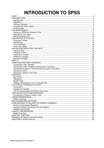
Table of ContentsIntroduction to SPSS .3One-sample t test 16Sample SPSS annotation 18Independent samples t test . 19One-way ANOVA . .21Correlated groups t test . 24Repeated measures ANOVA . 26Correlation and regression . 30Chi square . 332 X 2 Factorial ANOVA 352 X 3 Factorial ANOVA 39—2—
SPSS: An IntroductionWelcome to your first experience with SPSS (Statistics Package for the Social Sciences). I hope you find thispacket useful as you begin to navigate your way through this statistics software package. You will refer to theseinstructions throughout the semester, but I highly recommend hanging on to the packet for use in future classesand (if you are a Psychology or Neuroscience concentrator) for your Senior Project.OverviewThis section of the packet will walk you through the following steps:1. Logging on to the Citrix server to access SPSS.2. Downloading a data file to your computer and uploading it to your SSS (student storage server) space.3. Opening a data file in SPSS and saving it to your computer or to your SSS space.4. Creating a data file in SPSS.5. Computing frequency tables and descriptive statistics and creating histograms/bar graphs using SPSS.6. Doing some basic data manipulations using SPSS (recoding variables, computing new variables).7. Ending your session with Citrix.PART 1: Logging on to the Citrix server to access SPSSSPSS for Windows is available via the Citrix server on any computer on campus, Macintosh or Windows.Consequently, you will be able to use SPSS on your own computer via the Citrix server. You will need to know yourusername and password for linking to the Citrix server, which should be the same as your e-mail username andpassword. The first time you use Citrix (and at the beginning of each academic year), you’ll need to register (it’s free).See ng-and-logging-into-citrix if you need help.1.Open your web browser and enter the following address: citrix.hamilton.edu. I recommend creating aBookmark called “Citrix” so you can easily navigate to it whenever you need to. Once you’ve registered(see above), you will be prompted to download and install the Citrix receiver client. If you have anydifficulty doing so, please see me.2.Once the client is installed, the Citrix Metaframe window will open when you go to the above address, andyou will be prompted for your username and password, which should be the same as your e-mail usernameand password (see Figure 1). After you type these, select the appropriate Domain: “students.hamilton.edu”and click on “Log On.”Figure 13.You should now see icons for the available software packages you can access through the Citrix server (seeFigure 2). You will be using SPSS. Find the correct icon and click on it.Figure 24.You will see a task progress window indicating that the application is starting. After a short lag (this couldtake up to 30 seconds or more), SPSS should be up and running and you can create a new data file or openan existing one. See instructions below in Part 3 for opening data files.
PART 2: Downloading the data file to the desktop and uploading it to your SSS space1. Open your web browser to the “My Hamilton” web page at the following fm).2. Log in using your email username and password.3. Click on the “Courses” tab, and in the column under “My Blackboard Courses,” click on the link to ourcourse. The Blackboard page for our class will open.4. Click on “Assignments” and you will see an item labeled “SPSS data file” with a link to a file calledGSS data 2016.sav. (GSS General Social Survey.) Click on the file and you will be prompted to save it. Youhave a couple of options here:a.Save the file to a folder for this course that you create on your laptop. Use this option if youplan to exclusively use your own laptop for data analysis in this course.b.Save the file to your SSS. This option is the most flexible, as you can then access it nomatter what computer you happen to be using. The easiest way to accomplish this is to temporarily store thefile on your local computer’s desktop and then upload it to your SSS via the “Files” tab on your MyHamilton page. A folder called “Citrix” is in your SSS (it gets created the first time you open SPSS usingCitrix) and there is a subfolder named “Documents” within that folder. Here is where you want to store allof your data files (see Figures 3 and 4 below). Once you’ve saved the file to your desktop, go to MyHamilton, choose the “Files” tab, click on “Citrix,” then “Documents,” and then choose “Upload File” toplace the data file in the documents folder within the Citrix folder on your SSS.Figure 3Figure 4
PART 3: Opening SPSS and saving your data file to your SSS spaceNote that you cannot simply double-click on an SPSS (.sav) file to open it. You must be within the SPSS programin order to open files. When SPSS is first opened, it will prompt you with the following window:Figure 5For the descriptive statistics project, you are using an existing data file, so select “Open another file ” in the“Recent Files:” box and then click “Open” at the bottom of the window (or just double-click “Open anotherfile ”). A window will open to allow you to navigate to the pre-existing data file.Figure 6Figure 7How to find your file:1. If you saved it to a folder on your laptop (see Figure 6): Click the down arrow on the menu bar and navigateto Local Disk H (see above left). Note that Local Disk C is your hard drive and H is you, signed into yourhard drive. It’s faster to just click H rather than having to click C, then find your username, then get to H.Once you’ve clicked on H, you can navigate to the folder where you stored your file (or to your desktop, ifyou just dumped it there). Click on the file and then click “open”. Your data file will open in SPSS.2. If you saved it to your SSS (see Figure 7): Click the down arrow on the menu bar and navigate to yourusername followed by (\\sss.hamilton.edu/users). (Note that mine is ESS for “Employee Storage Space” ratherthan SSS.) If you click on that, you’ll then see the Citrix folder and the documents folder into which yousaved your file earlier. Click on the file and then click “open”. Your data file will open in SPSS.Saving filesBe sure to save frequently so you don’t lose your work due to unforeseen circumstances. If you make changes tothe file, you can save an updated version of it by clicking on File in the SPSS menu bar, then Save As. A windowsimilar to that shown in Figure 6 or 7 will appear. Name your file with a meaningful, informative label, then click‘Save.’ A copy of your file will be saved in the folder you designate (either on your hard drive or on your SSS).File types in SPSS
Note that different SPSS file types have different extensions:.sav data file.spv output file.sps syntax file (written code for SPSS to execute; we won’t do much with syntax in this course, but you willbecome more familiar with it in subsequent courses. Note that any command you ask SPSS to run via the menuscan be pasted into a syntax file and saved for later use. This is very handy when you’re working on an actualresearch project.)If you click on the folder icon in a data window, SPSS will automatically try to open data. If you click on thefolder icon in an output window, SPSS will automatically try to open output. If you click on the folder icon in asyntax window, SPSS will automatically try to open syntax. If you are in a data window and want to open eitheran output or syntax file, you will need to go to File, Open, and then choose data, output, or syntax.PART 4: Creating a data file in SPSSWhen you open SPSS, one of your choices in the “New Files:” box is “New Dataset” (see Figure 5, above). Ifyou click that option, you will be presented with an untitled data file (see Figure 8). Note that this file looks like astandard spreadsheet.Figure 8Before you can analyze your data, you must first input them into this file. Notice that the rows are alreadynumbered and the columns are labeled “var.” At this stage, they are shaded blue because they have not beenactivated with data or variable names.As you get familiar with the format of this spreadsheet, you should recognize that each column represents avariable and each row represents a participant’s data for each variable. So each row represents the scores from oneparticular participant.Before entering your data into this data file window, you’ll need to do a couple things. First, you need to figureout what you’re going to call each variable, keeping in mind that SPSS won’t let you begin a variable name with anumber or use special characters, such as spaces. Next, you need to figure out what sort of information you’llenter for each variable. In some cases, both of these decisions might be easy; but in other cases, more thoughtmight be required. For instance, if one of the variables that you want to enter is the gender of the participant, youcan’t enter the words “male” and “female;” instead, you need to develop a code (a way to quantify the variable).So, you might decide that for the variable “gender,” you will use a “1” to represent male and a “0” to representfemale. Of course, for some variables (e.g., age), you won’t need a code, but will simply enter in the value theparticipant reports.Define each variable
You can examine your variables/data in two different screens or “views”: data view and variable view. In dataview, you see the basic spreadsheet depicted in Figure 8. In variable view, you can easily name and define yourvariables (see Figure 9). You can toggle back and forth between these two views by clicking on the appropriatebutton (see bottom left of the screen). You can also double-click on a “var” header in data view to automaticallytoggle to variable view.I recommend that your first variable always be participant ID (an arbitrary number you assign to each participantfor record-keeping purposes). Below is an illustration of the variable view with the first variable added. Notice thevariable label (Participant ID Number) in the “label” column. It is important to get in the habit of labeling yourvariables. Labels help remind you what each variable is, and they also print out in the output so you know whatyou’re looking at. The variable labels for the data set for the descriptive statistics project are going to be veryimportant in helping you understand what the survey items were.Figure 9Let’s say that you wanted your second variable to be participant gender. As with participant ID, you need toprovide a variable name (a short name, e.g., “gender”) and a variable label (a description of the variable toremind yourself of what the variable is; e.g., “participant gender”). For this variable, though, you’ll need toprovide value labels to indicate what different levels of your variable mean. To do so, simply click in theappropriate cell in the “values” column (i.e., the cell that appears in the “gender” row). A lightly shaded blue boxappears within the cell, and if you click on it, a large dialog box appears in the middle of the screen (see Figure10). See how I’ve indicated that “1” represents male participants and “0” represents female participants? You cansimply type the value in one box and the value label in the box beneath it. Then click on “Add.” Once you’veadded all your values and value labels, click “OK.”
Figure 10Determining the number of decimal places each variable hasIn addition to giving your variable a label and defining its values, you may find it convenient to choose thenumber of decimal places you want displayed for each variable. For instance, if your variable is “gender,” and thevalues are “1” and “0,” it might annoy you to have SPSS display “1.00” and “0.00” all the way down the column(the default is 2 decimal places). To change the number of decimal places displayed, simply click on theappropriate cell (e.g., the one in the “gender” row and the “decimals” column). Up and down arrows appear in theright-hand part of the cell, and you can simply click on the down arrow until you have 0 decimal places (or youcan type “0” directly).Repeat this process of defining and labeling for all of your variables. NOTE: You’re not entering any of theparticipants’ data yet; you’re only getting the data file set up by creating and labeling the variables.Setting missing valuesIn SPSS, if you leave a cell blank, you will simply get a period (“.”) in that cell, and it will not be included in anyof the data analyses. Sometimes it is useful to use a particular number to represent missing data (e.g., 99, as longas 99 is not a valid value for that variable), and then to alert SPSS that a 99 is a missing value. Note that invariable view, there is a column titled “Missing” that alerts you to all the missing values for each variable.Figure 11To define values as missing, click in the appropriate cell for that variable under the “Missing” column like youdid for the value labels. You will get a dialog box into which you can input the appropriate missing values for thatvariable. Note that the General Social Survey data set includes quite a lot of missing values. These values are notincorporated into calculations involving that variable (e.g., the “99s” wouldn’t get incorporated into a meaninvolving that variable).Entering data
Once you’ve defined all the variables you need, you’re ready to enter the actual data. Generally, it’s easiest toenter all the data from a single participant before moving on to the next participant. That is, work row by row. Ifind it easiest to use the numerical keypad on the right side of an external keyboard (laptops don’t have these,which is why I hate entering data from a laptop!).Just for illustrative purposes, in Figure 12 you see the first portion of a sample questionnaire data file, showing 12participants and their scores on the first several variables of a questionnaire.Figure 12Checking for errorsThis is one of the most important steps of entering and analyzing data. If you made any errors inputting thenumbers, it could wreak havoc with your analyses and your interpretation of the data. If the errors are big ornumerous, it could mean the difference between supporting and rejecting a hypothesis! Be VERY CAREFULwhenever you enter data, and always double-check everything.If you’ve conducted an online survey and have exported data from Qualtrics, you still need to double-check it forerrors. For instance, I have sometimes discovered that a scale that was supposed to range from 1 to 6 in Qualtricsactually exported as bizarre numbers instead: 23, 24, 25, 26, 27, 28 instead of 1, 2, 3, 4, 5, 6. This can happen ifyou make a lot of edits to a survey question by deleting options and then adding them. You can avoid this byrecoding the values in Qualtrics before exporting the data, but if you don’t notice until later, you will need torecode them in SPSS. The important point is that you need to NOTICE the error in order to correct it, soexamining your data is vital.PART 5: Exploring your data: Conducting basic statistical analyses using SPSSNow you’re ready to start taking a look at your data. Below are described some of the descriptive statistics orgraphing options you might be interested in using. Later in the semester, we’ll discuss how to use more advancedtechniques (e.g., t tests, ANOVAs, correlation, & regression).TIP: Changing display preferencesBefore running any analyses, click on the Edit menu, then scroll to the bottom and select Options. A windowwill appear where you will be able to tell SPSS that you want the Variable Lists in any analysis window todisplay the names of the variables (the default in SPSS is to display the labels, which can be cumbersome).Note in Figure 13 below how the variable names appear in the column, rather than long variable labels.Also: If you click on the Output tab in Options, you can specify that, in your output, you would like variablesshown as names & labels, and variable values shown as values & labels. (Do so in both the “Outline Labeling”section and the “Pivot Table Labeling” section on the left of the dialog box.)
The “Frequencies” CommandIf you want SPSS to print you a frequency distribution, go under the “Analyze” menu, scroll down to “DescriptiveStatistics,” and then choose “Frequencies.” You’ll get a window like the one in Figure 13.Figure 13On the left side is a list of all the variables in your data file. Simply click on one you want to examine, then clickthe arrow to pop them into the “Variable(s)” box.TIP: Selecting multiple variables at onceYou can select multiple variables at the same time by holding down the Control key while clicking on thevariable names with the mouse. Alternatively, if the variables you desire are listed in sequence in the data file,you may click on the first variable, hold down the Shift key and click on the last variable in the list that youwant to examine.Once you’ve selected the variables you’d like to examine, you need to decide what information you’d like. Thedefault is just the frequency tables (notice the check mark in the box labeled “Display frequency tables”). If youdon’t want frequency tables, you can click on the box to remove the checkmark. If you click on the “Statistics”button, you can choose which measures of central tendency & variability you want to use. REMEMBER: Youneed to figure out what level of measurement a particular variable represents before willy-nilly choosing statistics.For example, calculating a mean gender doesn’t make any sense, because gender is measured on a nominal scale.THE COMPUTER WILL DO WHATEVER YOU TELL IT TO DO, EVEN IF YOU TELL IT TO DOSOMETHING WRONG! So you have to make sure to choose your statistics wisely.Histograms & Bar GraphsIf you want to look at your data graphically, you might choose to have SPSS draw you a histogram or a bar graphof a particular variable. Remember, histograms are used for quantitative variables (e.g., height), whereas bargraphs are used for qualitative variables (e.g., gender). Simply click on the “Charts” button within the frequenciescommand and choose which type of graph you want.The “Descriptives” CommandAnother way to get basic descriptive statistics is to go under “Analyze,” “Descriptive Statistics,” “Descriptives.”Here you’ll get many of the same options as with the “Frequencies” command, only you won’t get a frequencytable. Use this command if you just want to get a quick mean and standard deviation for a bunch of variables atonce.
Moving back and forth between the data window and the output windowWhenever you ask SPSS to calculate something for you, you automatically get bumped into the output window(“SPSS viewer”) where the output from your commands (e.g., frequency tables, descriptive statistics, graphs) isdisplayed. To get back to the data window, simply go up to the “Window” menu, and scroll down until you seethe name of the data file. If you want to edit a graph, double-click on it in the output window and you will bebumped into the “Chart Editor.” Again, you can return to any other window by going up to the “Window” menu.KEYBOARD SHORTCUTS FOR TOGGLING BETWEEN OPEN WINDOWS: Toggling between windows within the same program: On a Macintosh computer, selecting Command (the tilde symbol, top left of your keyboard) will toggle back and forth between open windows within thesame program. (Sorry, Windows computers don’t have this functionality!) Toggling between different programs: This is useful for, say, going back and forth between SPSS andMicrosoft Word if you’re writing up your homework. Hold down Command tab on a Mac or Alt tab ona PC.Save, Save, and Save Again!I strongly recommend saving your data file and output file every couple of minutes. You don’t want to lose hoursof work in case of a computer crash or power outage. Save frequently.Printing OutputUnfortunately, SPSS output prints out in a ridiculously large font with very little information on each page.Printing output “as is” wastes a lot of trees. You can certainly save your output (.spv) files on your computer tolook at on your screen, but whenever I ask you to print output for assignments, please do the following:Take a screen grab copy of the relevant part of the output (Ctrl Command Shift 4 on a Mac; for PCs, use thesnipping tool) and paste it (Command v) into your Microsoft Word document. You can then re-size the image tomake it smaller to fit on your page.Alternatively, you can export your output as “rich text format,” which will open in Microsoft Word, but this isstill fairly cumbersome and uses more trees than necessary. If you can’t get the screen grab to work, though, youcan do this: From within the output window, go to the “File” menu and choose “Export.” You will see thewindow below (Figure 14). Choose “Word/RTF(*.doc)” as the type (which is the default), click “browse” todecide where to save the file, give the file a descriptive name, and click OK in the Export window. You can nowopen the saved file in Microsoft Word, reformat the tables if you wish, delete any unnecessary information, andthen print your output.Figure 14Figure 15
Part 6: Performing basic data manipulations and computing new variablesRecoding VariablesSometimes it’s useful to be able to combine existing categories of responses into broader categories. For example,in the 2016 General Social Survey, the income variable has very narrow categories (1 under 1,000; 2 1,000 2,999; 3 3,000- 3,999; 4 4,000 – 4,999, etc through 26 170,000 or over). Perhaps you don’t need 26different income categories, but would rather group them into more meaningful chunks. You could decide thatyou want the following categories instead:1 under 20,000 (this would encompass values 1 – 12 in the old variable)2 between 20,000 and 40,000 (values 13 – 17 in the old variable)3 between 40,000 and 60,000 (values 18 – 19 in the old variable)4 between 60,000 and 90,000 (values 20 – 21 in the old variable; note that there’s unfortunately not an evenbreak at 80,000 in the data set)5 between 90,000 and 130,000 (values 22 – 23 in the old variable)6 over 130,000 (values 24 – 26 in the old variable)To do this, you would need to recode the original values into new ones. The original values 1-12 would berecoded as a 1 (under 20,000) in the new variable. The original 13-17 would become 2, and so on. Toaccomplish this in SPSS, go up to the Transform menu and scroll down to Recode (see Figure 16).Figure 16You get two options: “Recode into same variables” and “Recode into different variables.” The former changes theexisting variable and the latter creates a new variable with the recoded values. I recommend always creating anew (different) variable and leaving the original intact. If you choose “Into different variables,” you will get thewindow you see below:Figure 17The names of all your variables will appear in the list on the left part of the window. Scroll down until you findthe variable(s) you’re looking for. In this case, I want to recode the INCOME variable. Simply click on thevariable you want, then click on the arrow (which will be pointing the opposite of the way it’s pointing in the
figure). Now you need to tell SPSS what you want the new (recoded) variables to be called. To make life easier, Iusually just add “r” to the original variable name, to remind myself that the variable has been recoded. In thiscase, income becomes income r. Type this new name in the “output variable” box on the right of the window andclick on the “Change” button.Now you’re ready to tell SPSS how to recode the variable. To do so, first click on the “Old and New Values” box.You’ll get the screen you see below. In this case, we want the first 12 income categories of the old variable tobecome a “1” in the new, recoded variable. Notice that in the dialog box below, I’ve defined a range from 1-12for “Old Value”. On the right, I’ve entered a 1 under “New Value”. You would then click on “Add,” and keepgoing with the rest of the recodes (e.g., 13-17 becomes a 2, 18-19 becomes a 3, etc.). When you’ve added all therecodes to the Old New box, click Continue.Figure 18This will take you back to the window in Figure 17, and you can simply click “OK.” If you now scroll to the endof your data file, you’ll find a new column there called income r. You can run a frequency on it (Analyze,Descriptive Statistics, Frequencies) to double-check that your categories look good.Recoding is useful in other instances as well. For instance, questionnaires are often constructed such thatapproximately half of the questions are framed positively and the other half are framed negatively. For example,the 2016 General Social Survey included 6 items from the Life Orientation Test – Revised, a measure of optimism(see below). These items are scored on a 5-point Likert-type scale, from 1 (strongly disagree) to 5 (stronglyagree). Note that items 2, 4, and 5 are reverse-worded, such that high numbers actually mean greater pessimismrather than greater optimism. Researchers generally want to combine items such as these into a single measure foranalysis (i.e., a single optimism score that represents the mean of each respondent’s rating for all six questions).To do so, we would first have to reverse-score the two reverse-worded items, so that higher numbers always meanhigher optimism.Figure 19We could do this in a similar way to how we recoded the income variable, above. To reverse the response scalefor items LOTR2, LOTR4, and LOTR5, we need to recode the values such that 1 5, 2 4, 3 3, 4 2, and 5 1.Since both variables are being recoded in the same way, we can put both of them in the box shown in Figure 17.When we click “Old and New Values,” we’ll get the following:
Figure 20Note that this time we’re recoding individual values rather than a range. Note how I’ve already recoded 1 into 5, 2into 4, 3 into 3 (probably unnecessary, but I do it just in case .), and 4 into 2, and am in the process of changing5 into 1.Computing a new variable from existing onesOnce you have recoded any reverse-worded items, you can compute what is known as a “composite variable” forthe questionnaire. That is, you will compute a variable that represents each participant’s mean of all thequestionnaire items. (Note: Technically you would only do this if you had ascertained that all of the variableswere highly intercorrelated with one another, but that’s a lesson for another course! Given that this is anestablished optimism scale, we’ll go ahead and compute the mean.)There are 6 items on the optimism scale, so if I wanted to compute each participant’s mean optimism score basedon those 6 items, I could use a compute statement. Don’t forget that we need to use the recoded items instead ofthe originals for questions 2, 4, and 5. To create our compute statement, we would go up to the Transform menuagain and scroll down to “Compute.” You should then see a window that looks like the one below:Figure 21Note how I’ve typed “LOTR mean” in the “Target Variable” box. That means I want SPSS to create a newcolumn labeled “LOTR mean” that will represent each participant’s mean on the optimism scale. In the “NumericExpression” box, I’ve indicated that I want this new variable to equal the mean of the items on the optimismscale, substituting the recoded items for the originals where appropriate. When you’re all set, click “OK.” If youscroll to the end of the data file, you’ll see a new column labeled “LOTR mean.” This variable would representeach participant’s average optimism score based on the 6-item questionnaire.NOTE: You can use the compute command to perform any of a number of functions. I’ve chosen to calculate amean.
TIP: Pasting syntax. If you wanted to save this formula to use again later, you could click “Paste,” and theformula would get pasted into the Syntax window, where you could run the command by highlighting it andclicking the green “go” button, and could also save it for later use.Play around! Explore! Have fun!SPSS is a fairly user-friendly program. If you get lost, simply scroll around in the menus until you find whatyou’re looking for. If you’re really lost, you can probably Google for help. Remember, though: SPSS will blindlydo whatever you tell it to do, regardless of whether or not it’s a sensible command. So be smart about what youtell it to do. Now you’re ready to explore your data. Enjoy!Part 7: Ending your session with CitrixWhen you are done working, remember to save your files. From within SPSS, choose File, then Exit. This willautomatically log you off of Citrix as well. (If you forget to do this and instead quit Citrix without first quittingSPSS, it is very important to select log off rather than disconnect so you don’t have multiple Citrix sessions open.)
SPSS Instructions for a One-Sample t TestWe will use data from a class questionnaire distributed in a previous semester of Psych Stats to illustrate how toconduct a one-sample t test. We will examine the number of hours of sleep per week that students get, andwhether this number differs significantly from the recommended 8 hours. The first several cases of the file appearas follows:Figure 1To conduct a one-sample t test in SPSS, go to the “Analyze” menu and click on “Compare means” and then “OneSample T Test.” Click on the DV you want to analyze (in this case, “sleep hrs week”) and click on the arrow toput it in the “Test Variable(s)” box (see Figure 2).Figure 2Next, you need to decide what your test value is going to be. This is the value to which you willcompare the overall mean of the distribution. For our example, the test value is 8 hours, as we w
Note that different SPSS file types have different extensions:.sav data file.spv output file.sps syntax file (written code for SPSS to execute; we won't do much with syntax in this course, but you will become more familiar with it in subsequent courses. Note that any command you ask SPSS to run via the menus