![Optimization Models [.1] Exercises - People](/img/36/exmanual.jpg)
Transcription
GIUSEPPE CALAFIOREANDL AU R E N T E L G H AO U IO P T I M I Z AT I O N M O D E L SEXERCISESCAMBRIDGE
Contents2.Vectors3.Matrices4.Symmetric matrices5.Singular Value Decomposition6.Linear Equations7.Matrix Algorithms8.Convexity9.Linear, Quadratic and Geometric Models47111621263010. Second-Order Cone and Robust Models11. Semidefinite Models4412. Introduction to Algorithms13. Learning from Data5714. Computational Finance15. Control Problems16. Engineering Design516171753540
42.VectorsExercise 2.1 (Subpaces and dimensions) Consider the set S of pointssuch thatx1 2x2 3x3 0, 3x1 2x2 x3 0.Show that S is a subspace. Determine its dimension, and find a basisfor it.Exercise 2.2 (Affine sets and projections) Consider the set in R3 defined by the equationnoP x R3 : x1 2x2 3x3 1 .1. Show that the set P is an affine set of dimension 2. To this end,express it as x (0) span( x (1) , x (2) ), where x (0) P , and x (1) , x (2)are linearly independent vectors.2. Find the minimum Euclidean distance from 0 to the set P , and apoint that achieves the minimum distance.Exercise 2.3 (Angles, lines and projections)1. Find the projection z of the vector x (2, 1) on the line that passesthrough x0 (1, 2) and with direction given by vector u (1, 1).2. Determine the angle between the following two vectors: 31 x 2 , y 2 .13Are these vectors linearly independent?Exercise 2.4 (Inner product) Let x, y Rn . Under which conditionon α Rn does the functionnf ( x, y) αk xk ykk 1define an inner product on Rn ?Exercise 2.5 (Orthogonality) Let x, y Rn be two unit-norm vectors,that is, such that k x k2 kyk2 1. Show that the vectors x y andx y are orthogonal. Use this to find an orthogonal basis for thesubspace spanned by x and y.Exercise 2.6 (Norm inequalities)
51. Show that the following inequalities hold for any vector x: 1 k x k2 k x k k x k2 k x k1 n k x k2 n k x k .nHint: use the Cauchy–Schwartz inequality.2. Show that for any nonzero vector x,card( x ) k x k21,k x k22where card( x ) is the cardinality of the vector x, defined as the number of nonzero elements in x. Find vectors x for which the lowerbound is attained.Exercise 2.7 (Hölder inequality) Prove Hölder’s inequality (2.4).Hint: consider the normalized vectors u x/k x k p , v y/kykq ,and observe that x y k x k p k y k q · u v k x k p k y k q u k v k .kThen, apply Young’s inequality (see Example 8.10) to the products uk vk uk vk .Exercise 2.8 (Linear functions)1. For a n-vector x, with n 2m 1 odd, we define the median ofx as the scalar value x a such that exactly n of the values in x are x a and n are x a (i.e., x a leaves half of the values in x to its left,and half to its right). Now consider the function f : Rn R, withvalues f ( x ) x a n1 in 1 xi . Express f as a scalar product, that is,find a Rn such that f ( x ) a x for every x. Find a basis for theset of points x such that f ( x ) 0.2. For α R2 , we consider the “power law” function f : R 2 R,αwith values f ( x ) x1 1 x2α2 . Justify the statement: “the coefficientsαi provide the ratio between the relative error in f to a relativeerror in xi ”.Exercise 2.9 (Bound on a polynomial’s derivative) In this exercise,you derive a bound on the largest absolute value of the derivativeof a polynomial of a given order, in terms of the size of the coefficients.1 For w Rk 1 , we define the polynomial pw , with values.p w ( x ) w1 w2 x · · · w k 1 x k .See the discussion on regularizationin Section 13.2.3 for an application ofthis result.1
6Show that, for any p 1 x [ 1, 1] :dpw ( x ) C (k, p)kvk p ,dxwhere v (w2 , . . . , wk 1 ) Rk , and kk3/2C (k, p) k ( k 1)2p 1,p 2,p .Hint: you may use Hölder’s inequality (2.4) or the results from Exercise 2.6.
73.MatricesExercise 3.1 (Derivatives of composite functions)1. Let f : Rm Rk and g : Rn Rm be two maps. Let h : Rn Rkbe the composite map h f g, with values h( x ) f ( g( x )) forx Rn . Show that the derivatives of h can be expressed via amatrix–matrix product, as Jh ( x ) J f ( g( x )) · Jg ( x ), where Jh ( x ) isthe Jacobian matrix of h at x, i.e., the matrix whose (i, j) element hi ( x )is x.j2. Let g be an affine map of the form g( x ) Ax b, for A Rm,n ,b Rm . Show that the Jacobian of h( x ) f ( g( x )) isJh ( x ) J f ( g( x )) · A.3. Let g be an affine map as in the previous point, let f : Rn R (ascalar-valued function), and let h( x ) f ( g( x )). Show that x h( x ) 2x h( x ) A g f ( g( x )),A 2g f ( g( x )) A.Exercise 3.2 (Permutation matrices) A matrix P Rn,n is a permutation matrix if its columns are a permutation of the columns of then n identity matrix.1. For an n n matrix A, we consider the products PA and AP. Describe in simple terms what these matrices look like with respectto the original matrix A.2. Show that P is orthogonal.Exercise 3.3 (Linear maps) Let f : Rn Rm be a linear map. Showhow to compute the (unique) matrix A such that f ( x ) Ax for everyx Rn , in terms of the values of f at appropriate vectors, which youwill determine.Exercise 3.4 (Linear dynamical systems) Linear dynamical systemsare a common way to (approximately) model the behavior of physicalphenomena, via recurrence equations of the form2x (t 1) Ax (t) Bu(t), y(t) Cx (t), t 0, 1, 2, . . . ,where t is the (discrete) time, x (t) Rn describes the state of thesystem at time t, u(t) R p is the input vector, and y(t) Rm is theoutput vector. Here, matrices A, B, C, are given.Such models are the focus of Chapter 15.2
81. Assuming that the system has initial condition x (0) 0, express the output vector at time T as a linear function of u(0), . . .,u( T 1); that is, determine a matrix H such that y( T ) HU ( T ),where u (0) . . U (T ) . u ( T 1)contains all the inputs up to and including at time T 1.2. What is the interpretation of the range of H?Exercise 3.5 (Nullspace inclusions and range) Let A, B Rm,n betwo matrices. Show that the fact that the nullspace of B is containedin that of A implies that the range of B contains that of A .Exercise 3.6 (Rank and nullspace) Consider the image in Figure 3.1,a gray-scale rendering of a painting by Mondrian (1872–1944). Webuild a 256 256 matrix A of pixels based on this image by ignoringgrey zones, assigning 1 to horizontal or vertical black lines, 2 atthe intersections, and zero elsewhere. The horizontal lines occur atrow indices 100, 200 and 230, and the vertical ones at columns indices50, 230.1. What is nullspace of the matrix?2. What is its rank?Exercise 3.7 (Range and nullspace of A A) Prove that, for any matrix A Rm,n , it holds thatN ( A A ) N ( A ),R ( A A ) R ( A ).(3.1)Hint: use the fundamental theorem of linear algebra.Exercise 3.8 (Cayley–Hamilton theorem) Let A Rn,n and let.p(λ) det(λIn A) λn cn 1 λn 1 · · · c1 λ c0be the characteristic polynomial of A.1. Assume A is diagonalizable. Prove that A annihilates its owncharacteristic polynomial, that isp( A) An cn 1 An 1 · · · c1 A c0 In 0.Hint: use Lemma 3.3.Figure 3.1: A gray-scale rendering ofa painting by Mondrian.
92. Prove that p( A) 0 holds in general, i.e., also for non-diagonalizable square matrices. Hint: use the facts that polynomials arecontinuous functions, and that diagonalizable matrices are densein Rn,n , i.e., for any e 0 there exist Rn,n with k kF e suchthat A is diagonalizable.Exercise 3.9 (Frobenius norm and random inputs) Let A Rm,n bea matrix. Assume that u Rn is a vector-valued random variable,with zero mean and covariance matrix In . That is, E{u} 0, andE{uu } In .1. What is the covariance matrix of the output, y Au?2. Define the total output variance as E{ky ŷk22 }, where ŷ E{y}is the output’s expected value. Compute the total output varianceand comment.Exercise 3.10 (Adjacency matrices and graphs) For a given undirected graph G with no self-loops and at most one edge between anypair of nodes (i.e., a simple graph), as in Figure 3.2, we associate an n matrix A, such thatAij (1 if there is an edge between node i and node j,0 otherwise.This matrix is called the adjacency matrix of the graph.31. Prove the following result: for positive integer k, the matrix Akhas an interesting interpretation: the entry in row i and column jgives the number of walks of length k (i.e., a collection of k edges)leading from vertex i to vertex j. Hint: prove this by induction onk, and look at the matrix–matrix product Ak 1 A.2. A triangle in a graph is defined as a subgraph composed of threevertices, where each vertex is reachable from each other vertex(i.e., a triangle forms a complete subgraph of order 3). In thegraph of Figure 3.2, for example, nodes {1, 2, 4} form a triangle.Show that the number of triangles in G is equal to the trace of A3divided by 6. Hint: For each node in a triangle in an undirectedgraph, there are two walks of length 3 leading from the node toitself, one corresponding to a clockwise walk, and the other to acounter-clockwise walk.Exercise 3.11 (Nonnegative and positive matrices) A matrix A Rn,nis said to be non-negative (resp. positive) if aij 0 (resp. aij 0) for21354Figure 3.2: An undirected graph withn 5 vertices.3The graph incency matrix 0 1 A 0 11Figure 3.2 has adja10011000011100011100 .
10all i, j 1, . . . , n. The notation A 0 (resp. A 0) is used to denotenon-negative (resp. positive) matrices.A non-negative matrix is said to be column (resp. row) stochastic,if the sum of the elements along each column (resp. row) is equal toone, that is if 1 A 1 (resp. A1 1). Similarly, a vector x Rnis said to be non-negative if x 0 (element-wise), and it is said tobe a probability vector, if it is non-negative and 1 x 1. The set ofprobability vectors in Rn is thus the set S { x Rn : x 0, 1 x 1}, which is called the probability simplex. The following points youare requested to prove are part of a body of results known as thePerron–Frobenius theory of non-negative matrices.1. Prove that a non-negative matrix A maps non-negative vectorsinto non-negative vectors (i.e., that Ax 0 whenever x 0), andthat a column stochastic matrix A 0 maps probability vectorsinto probability vectors.2. Prove that if A 0, then its spectral radius ρ( A) is positive. Hint:use the Cayley–Hamilton theorem.3. Show that it holds for any matrix A and vector x that Ax A x ,where A (resp. x ) denotes the matrix (resp. vector) of moduliof the entries of A (resp. x). Then, show that if A 0 and λi , vi isan eigenvalue/eigenvector pair for A, then λi vi A vi .4. Prove that if A 0 then ρ( A) is actually an eigenvalue of A (i.e., Ahas a positive real eigenvalue λ ρ( A), and all other eigenvaluesof A have modulus no larger than this “dominant” eigenvalue),and that there exist a corresponding eigenvector v 0. Further,the dominant eigenvalue is simple (i.e., it has unit algebraic multiplicity), but you are not requested to prove this latter fact.Hint: For proving this claim you may use the following fixed-pointtheorem due to Brouwer: if S is a compact and convex set4 in Rn , andf : S S is a continuous map, then there exist an x S such that.f ( x ) x. Apply this result to the continuous map f ( x ) 1 AxAx ,with S being the probability simplex (which is indeed convex andcompact).5. Prove that if A 0 and it is column or row stochastic, then itsdominant eigenvalue is λ 1.See Section 8.1 for definitions ofcompact and convex sets.4
114.Symmetric matricesExercise 4.1 (Eigenvectors of a symmetric 2 2 matrix) Let p, q Rnbe two linearly independent vectors, with unit norm (k pk2 kqk2 .1). Define the symmetric matrix A pq qp . In your derivations,.it may be useful to use the notation c p q.1. Show that p q and p q are eigenvectors of A, and determinethe corresponding eigenvalues.2. Determine the nullspace and rank of A.3. Find an eigenvalue decomposition of A, in terms of p, q. Hint: usethe previous two parts.4. What is the answer to the previous part if p, q are not normalized?Exercise 4.2 (Quadratic constraints) For each of the following cases,determine the shape of the region generated by the quadratic constraint x Ax 1."#2 11. A .1 22. A "3. A " 11#. 1 00 1#.1 1Hint: use the eigenvalue decomposition of A, and discuss dependingon the sign of the eigenvalues.Exercise 4.3 (Drawing an ellipsoid)1. How would you efficiently draw an ellipsoid in R2 , if the ellipsoidis described by a quadratic inequality of the formnoE x Ax 2b x c 0 ,where A is 2 2 and symmetric, positive definite, b R2 , andc R? Describe your method as precisely as possible.2. Draw the ellipsoidnoE 4x12 2x22 3x1 x2 4x1 5x2 3 1 .
12Exercise 4.4 (Minimizing a quadratic function) Consider the unconstrained optimization problemp minx1 x Qx c x2where Q Q Rn,n , Q 0, and c Rn are given. The goal of thisexercise is to determine the optimal value p and the set of optimalsolutions, X opt , in terms of c and the eigenvalues and eigenvectorsof the (symmetric) matrix Q.1. Assume that Q 0. Show that the optimal set is a singleton, andthat p is finite. Determine both in terms of Q, c.2. Assume from now on that Q is not invertible. Assume furtherthat Q is diagonal: Q diag (λ1 , . . . , λn ), with λ1 . . . λr λr 1 . . . λn 0, where r is the rank of Q (1 r n). Solvethe problem in that case (you will have to distinguish between twocases).3. Now we do not assume that Q is diagonal anymore. Under whatconditions (on Q, c) is the optimal value finite? Make sure to express your result in terms of Q and c, as explicitly as possible.4. Assuming that the optimal value is finite, determine the optimalvalue and optimal set. Be as specific as you can, and express yourresults in terms of the pseudo-inverse5 of Q.Exercise 4.5 (Interpretation of covariance matrix) As in Example 4.2,we are given m points x (1) , . . . , x (m) in Rn , and denote by Σ the sample covariance matrix:. 1Σ mwhere x̂ Rnm (x(i) x̂)(x(i) x̂) ,i 1is the sample average of the points:. 1x̂ mm x (i ) .i 1We assume that the average and variance of the data projected alonga given direction does not change with the direction. In this exercisewe will show that the sample covariance matrix is then proportionalto the identity.We formalize this as follows. To a given normalized directionw Rn , kwk2 1, we associate the line with direction w passingthrough the origin, L(w) {tw : t R }. We then consider theprojection of the points x (i) , i 1, . . . , m, on the line L(w), and look5See Section 5.2.3.
13at the associated coordinates of the points on the line. These projectedvalues are given by.ti (w) arg min ktw x (i) k2 , i 1, . . . , m.tWe assume that for any w, the sample average t̂(w) of the projectedvalues ti (w), i 1, . . . , m, and their sample variance σ2 (w), are bothconstant, independent of the direction w. Denote by t̂ and σ2 the(constant) sample average and variance. Justify your answer to thefollowing questions as carefully as you can.1. Show that ti (w) w x (i) , i 1, . . . , m.2. Show that the sample average x̂ of the data points is zero.3. Show that the sample covariance matrix Σ of the data points isof the form σ2 In . Hint: the largest eigenvalue λmax of the matrixΣ can be written as: λmax maxw {w Σw : w w 1}, and asimilar expression holds for the smallest eigenvalue.Exercise 4.6 (Connected graphs and the Laplacian) We are given agraph as a set of vertices in V {1, . . . , n}, with an edge joining anypair of vertices in a set E V V. We assume that the graph isundirected (without arrows), meaning that (i, j) E implies ( j, i ) E. As in Section 4.1, we define the Laplacian matrix by 1 if (i, j) E,Lij d(i ) if i j, 0otherwise.Picture 1.png 250 165 pixelsFigure 4.3: Example of an undirectedgraph.Here, d(i ) is the number of edges adjacent to vertex i. For example,d(4) 3 and d(6) 1 for the graph in Figure 4.3.1. Form the Laplacian for the graph shown in Figure 4.3.2. Turning to a generic graph, show that the Laplacian L is symmetric.3. Show that L is positive-semidefinite, proving the following identity, valid for any u Rn :. 1u Lu q(u) ( u i u j )2 .2 (i,j ) EHint: find the values q(k), q(ek el ), for two unit vectors ek , el suchthat (k, l ) E.4. Show that 0 is always an eigenvalue of L, and exhibit an eigenvector. Hint: consider a matrix square-root6 of L.6See Section 1.png
145. The graph is said to be connected if there is a path joining anypair of vertices. Show that if the graph is connected, then the zeroeigenvalue is simple, that is, the dimension of the nullspace of Lis 1. Hint: prove that if u Lu 0, then ui u j for every pair(i, j) E.Exercise 4.7 (Component-wise product and PSD matrices) Let A, B Sn be two symmetric matrices. Define the component-wise productof A, B, by a matrix C Sn with elements Cij Aij Bij , 1 i, j n.Show that C is positive semidefinite, provided both A, B are. Hint:prove the result when A is rank-one, and extend to the general casevia the eigenvalue decomposition of A.Exercise 4.8 (A bound on the eigenvalues of a product) Let A, B Sn be such that A 0, B 0.1. Show that all eigenvalues of BA are real and positive (despite thefact that BA is not symmetric, in general). . 2. Let A 0, and let B 1 diag k a1 k1 , . . . , k a n k1 , where ai ,i 1, . . . , n, are the rows of A. Prove that0 λi ( BA) 1, i 1, . . . , n.3. With all terms defined as in the previous point, prove thatρ( I αBA) 1, α (0, 2).Exercise 4.9 (Hadamard’s inequality) Let A Sn be positive semidefinite. Prove thatndet A aii .i 1Hint: Distinguish the cases det A 0 and det A 6 0. In the lat.ter case,consider the normalized matrix à DAD, where D 1/21/2diag a11, . . . , a , and use the geometric–arithmetic mean innnequality (see Example 8.9).Exercise 4.10 (A lower bound on the rank) Let A Sn be a symmetric, positive semidefinite matrix.1. Show that the trace, trace A, and the Frobenius norm, k AkF , depend only on its eigenvalues, and express both in terms of thevector of eigenvalues.2. Show that(trace A)2 rank( A)k Ak2F .
153. Identify classes of matrices for which the corresponding lowerbound on the rank is attained.Exercise 4.11 (A result related to Gaussian distributions) Let Σ Sn be a symmetric, positive definite matrix. Show thatZ1 Σ 1 xRne 2 x dx (2π )n/2 det Σ.You may assume known that the result holds true when n 1. Theabove shows that the function p : Rn R with (non-negative) values1 11 p( x ) e 2 x Σ x(2π )n/2 · det Σintegrates to one over the whole space. In fact, it is the density function of a probability distribution called the multivariate Gaussian (ornormal) distribution, with zero mean and covariance matrix Σ. Hint:you may use the fact that for any integrable function f , and invertiblen n matrix P, we haveZx Rnf ( x )dx det P ·Zz Rnf ( Pz)dz.
165.Singular Value DecompositionExercise 5.1 (SVD of an orthogonal matrix) 1 221 A 2 1 2322 11. Show that A is orthogonal.Consider the matrix .2. Find a singular value decomposition of A.Exercise 5.2 (SVD of a matrix with orthogonal columns) Assume amatrix A [ a1 , . . . , am ] has columns ai Rn , i 1, . . . , m that areorthogonal to each other: ai a j 0 for 1 i 6 j n. Find an SVDfor A, in terms of the ai s. Be as explicit as you can.Exercise 5.3 (Singular values of augmented matrix) Let A Rn,m ,with n m, have singular values σ1 , . . . , σm .1. Show that the singular values of the (n m) m matrix"#A.Ã Imare σ̃i q1 σi2 , i 1, . . . , m.2. Find an SVD of the matrix Ã.Exercise 5.4 (SVD of score matrix) An exam with m questions is given to n students. The instructor collects all the grades in a n mmatrix G, with Gij the grade obtained by student i on question j. Wewould like to assign a difficulty score to each question, based on theavailable data.1. Assume that the grade matrix G is well approximated by a rankone matrix sq , with s Rn and q Rm (you may assume thatboth s, q have non-negative components). Explain how to use theapproximation to assign a difficulty level to each question. Whatis the interpretation of vector s?2. How would you compute a rank-one approximation to G? Stateprecisely your answer in terms of the SVD of G.Exercise 5.5 (Latent semantic indexing) Latent semantic indexing isan SVD-based technique that can be used to discover text documentssimilar to each other. Assume that we are given a set of m documents D1 , . . . , Dm . Using a “bag-of-words” technique described in
17Example 2.1, we can represent each document D j by an n-vector d j ,where n is the total number of distinct words appearing in the wholeset of documents. In this exercise, we assume that the vectors d jare constructed as follows: d j (i ) 1 if word i appears in documentD j , and 0 otherwise. We refer to the n m matrix M [d1 , . . . , dm ]as the “raw” term-by-document matrix. We will also use a normalized7 version of that matrix: M̃ [d 1 , . . . , d m ], where d j d j /kd j k2 ,j 1, . . . , m.Assume we are given another document, referred to as the “querydocument,” which is not part of the collection. We describe thatquery document as an n-dimensional vector q, with zeros everywhere, except a 1 at indices corresponding to the terms that appearin the query. We seek to retrieve documents that are “most similar”to the query, in some sense. We denote by q̃ the normalized vectorq̃ q/kqk2 .In practice, other numerical representation of text documents can beused. For example we may use therelative frequencies of words in eachdocument, instead of the 2 -normnormalization employed here.71. A first approach is to select the documents that contain the largestnumber of terms in common with the query document. Explainhow to implement this approach, based on a certain matrix–vectorproduct, which you will determine.2. Another approach is to find the closest document by selecting theindex j such that kq d j k2 is the smallest. This approach canintroduce some biases, if for example the query document is muchshorter than the other documents. Hence a measure of similaritybased on the normalized vectors, kq̃ d j k2 , has been proposed,under the name of “cosine similarity”. Justify the use of this namefor that method, and provide a formulation based on a certainmatrix–vector product, which you will determine.3. Assume that the normalized matrix M̃ has an SVD M̃ UΣV ,with Σ an n m matrix containing the singular values, and theunitary matrices U [u1 , . . . , un ], V [v1 , . . . , vm ] of size n n,m m respectively. What could be an interpretation of the vectorsul , vl , l 1, . . . , r? Hint: discuss the case when r is very small, andthe vectors ul , vl , l 1, . . . , r, are sparse.4. With real-life text collections, it is often observed that M is effectively close to a low-rank matrix. Assume that a optimal rank-kapproximation (k min(n, m)) of M̃, M̃k , is known. In the latentsemantic indexing approach8 to document similarity, the idea is tofirst project the documents and the query onto the subspace generated by the singular vectors u1 , . . . , uk , and then apply the cosinesimilarity approach to the projected vectors. Find an expressionfor the measure of similarity.In practice, it is often observed thatthis method produces better resultsthan cosine similarity in the originalspace, as in part 2.8
18Exercise 5.6 (Fitting a hyperplane to data) We are given m data pointsd1 , . . . , dm Rn , and we seek a hyperplane.H(c, b) { x Rn : c x b},where c Rn , c 6 0, and b R, that best “fits” the given points,in the sense of a minimum sum of squared distances criterion, seeFigure 5.4.Formally, we need to solve the optimization problemmminc,b43210 1 2 3 4 3 dist2i 1(di , H(c, b)) : kck2 1,where dist(d, H) is the Euclidean distance from a point d to H. Herethe constraint on c is imposed without loss of generality, in a waythat does not favor a particular direction in space.1. Show that the distance from a given point d Rn to H is given bydist(d, H(c, b)) c d b .2. Show that the problem can be expressed asminb,c : kck2 1f 0 (b, c),where f 0 is a certain quadratic function, which you will determine.3. Show that the problem can be reduced tominc ( D̃ D̃ )cs.t.:kck2 1,cwhere D̃ is the matrix of centered data points: the i-th column of.D̃ is di d, where d (1/m) im 1 di is the average of the datapoints. Hint: you can exploit the fact that at optimum, the partialderivative of the objective function with respect to b must be zero,a fact justified in Section 8.4.1.4. Explain how to find the hyperplane via SVD.Exercise 5.7 (Image deformation) A rigid transformation is a mapping from Rn to Rn that is the composition of a translation and arotation. Mathematically, we can express a rigid transformation φ asφ( x ) Rx r, where R is an n n orthogonal transformation andr Rn a vector. 2 10123Figure 5.4: Fitting a hyperplane todata.
19We are given a set of pairs of points ( xi , yi ) in Rn , i 1, . . . , m,and wish to find a rigid transformation that best matches them. Wecan write the problem asmminn,nR R, r Rn k Rxi r yi k22: R R In ,(5.2)i 1where In is the n n identity matrix.The problem arises in image processing, to provide ways to deform an image (represented as a set of two-dimensional points) basedon the manual selection of a few points and their transformed counterparts.1. Assume that R is fixed in problem (5.2). Express an optimal r as afunction of R.2. Show that the corresponding optimal value (now a function of Ronly) can be written as the original objective function, with r 0and xi , yi replaced with their centered counterparts,x̄i xi x̂, x̂ 1mm xj,j 1ȳi yi ŷ, ŷ 1mm yj.j 13. Show that the problem can be written asmin k RX Y kF : R R In ,Rfor appropriate matrices X, Y, which you will determine. Hint:explain why you can square the objective; then expand.4. Show that the problem can be further written asmax trace RZ : R R In ,Rfor an appropriate n n matrix Z, which you will determine.5. Show that R VU is optimal, where Z USV is the SVD ofZ. Hint: reduce the problem to the case when Z is diagonal, anduse without proof the fact that when Z is diagonal, In is optimalfor the problem.6. Show the result you used in the previous question: assume Z isdiagonal, and show that R In is optimal for the problem above.Hint: show that R R In implies Rii 1, i 1, . . . , n, andusing that fact, prove that the optimal value is less than or equalto trace Z.Figure 5.5: Image deformation viarigid transformation. The image onthe left is the original image, and thaton the right is the deformed image.Dots indicate points for which the deformation is chosen by the user.
207. How woud you apply this technique to make Mona Lisa smilemore? Hint: in Figure 5.5, the two-dimensional points xi are given(as dots) on the left panel, while the corresponding points yi areshown on the left panel. These points are manually selected. Theproblem is to find how to transform all the other points in theoriginal image.
216.Linear EquationsExercise 6.1 (Least squares and total least squares) Find the leastsquares line and the total least-squares9 line for the data points ( xi , yi ),i 1, . . . , 4, with x ( 1, 0, 1, 2), y (0, 0, 1, 1). Plot both lines onthe same set of axes.Exercise 6.2 (Geometry of least squares) Consider a least-squaresproblemp min k Ax yk2 ,xwhere A y We assume that y 6 R( A), so that p 0.Show that, at optimum, the residual vector r y Ax is such thatr y 0, A r 0. Interpret the result geometrically. Hint: use theSVD of A. You can assume that m n, and that A is full columnrank.Rm,n ,Rm .Exercise 6.3 (Lotka’s law and least squares) Lotka’s law describesthe frequency of publication by authors in a given field. It statesthat X a Y b, where X is the number of publications, Y the relativefrequency of authors with X publications, and a and b are constants(with b 0) that depend on the specific field. Assume that we havedata points ( Xi , Yi ), i 1, . . . , m, and seek to estimate the constants aand b.1. Show how to find the values of a, b according to a linear leastsquares criterion. Make sure to define the least-squares probleminvolved precisely.2. Is the solution always unique? Formulate a condition on the datapoints that guarantees unicity.Exercise 6.4 (Regularization for noisy data) Consider a least-squaresproblemmin k Ax yk22 ,xin which the data matrix A Rm,n is noisy. Our specific noise modelassumes that each row ai Rn has the form ai âi ui , wherethe noise vector ui Rn has zero mean and covariance matrix σ2 In ,with σ a measure of the size of the noise. Therefore, now the matrixA is a function of the uncertain vector u (u1 , . . . , un ), which wedenote by A(u). We will write  to denote the matrix with rows âi ,i 1, . . . , m. We replace the original problem withmin Eu {k A(u) x yk22 },x9See Section 6.7.5.
22where Eu denotes the expected value with respect to the randomvariable u. Show that this problem can be written asmin k Âx yk22 λk x k22 ,xwhere λ 0 is some regularization parameter, which you will determine. That is, regularized least squares can be interpreted as a wayto take into account uncertainties in the matrix A, in the expectedvalue sense. Hint: compute the expected value of (( âi ui ) x yi )2 ,for a specific row index i.Exercise 6.5 (Deleting a measurement in least squares) In this exercise, we revisit S
Contents 2.Vectors 4 3.Matrices 7 4.Symmetric matrices 11 5.Singular Value Decomposition 16 6.Linear Equations 21 7.Matrix Algorithms 26 8.Convexity 30 9.Linear, Quadratic and Geometric Models 35 10.Second-Order Cone and Robust Models 40 11.Semidefinite Models 44 12.Introduction to Algorithms 51 13.Learning from Data 57 14.Computational Finance 61 15.Control Problems 71 16.Engineering Design 75