Transcription
Machine Learning and OptimizationAndres MunozCourant Institute of Mathematical Sciences, New York, NY.Abstract. This final project attempts to show the differences of machine learning and optimization. In particular while optimization is concerned with exact solutions machine learning is concerned with generalization abilities of learners. We present examples in the areas of classification and regression where this difference is easy to observe as well astheoretical reasons of why this two areas are different even when theyseem similar at a first glance.1IntroductionSince the invention of computers people have been trying to answer thequestion of whether a computer can ‘learn’, and before we start talkingabout theorems and algorithms we should define what ‘learning’ meansfor a machine. Arthur Samuel in 1959 defined machine learning as the“field of study that gives computers the ability to learn without beingexplicitly programmed”. At the beginning this field was mainly algorithmic and without much foundations, it was probably thanks to the workof Valiant [6] who introduced the framework of PAC learning (probably approximately correct learning) that a real theory of the learnablewas established. Another milestone in the theory of learning was set byVapnik in [7]. Vapnik casts the problem of ‘learning’ as an optimizationproblem allowing people to use all of the theory of optimization that wasalready given. Nowadays machine learning is a combination of severaldisciplines such as statistics, information theory, theory of algorithms,probability and functional analysis. But as we will see optimization isstill at the heart of all modern machine learning problems. The layoutof the paper is as follows. First we present the definitions and notation needed, then we give a mathematical definition of learning and wegive the general optimization problem. In section 3 we present learningguarantees and describe the principle of empirical risk minimization. Inthe end we present experiments comparing the raw use of optimizationversus a combination of optimization and learning bounds.2DefinitionsWe will consider the following spaces: a space of examples X a space oflabels Y and a space of hypothesis H that contains functions mappingX to Y. We will also consider a loss function L : Y Y R and aprobability measure P over the space X Y.
Definition 1. For any hypothesis h H we define the risk of h withrespect to L and P to be:LP (h) E(L(h(x), y))PThe general problem of machine learning can be then cast as finding thehypothesis h H that solves the following optimization problem:min LP (h)h HBy having access only to a labeled sample S (xi , yi )ni 1 X Y. Asimplification of this scenario is given when the distribution P is givenonly over the example space X and there exists a labeling function f :X Y in that case we are trying to find a hypothesis h such that itsolves the optimization problem:min E(L(h(x), f (x))h H PExample 1. Consider X R2 and Y { 1, 1}, suppose there’s a probability distribution Px over X and that the labeling function f is anindicator function for a rectangle R R2 ,i.e: 1 x Rf (x) 1 x /RIf the loss function is the 0 1 loss i.e L(y, y 0 ) 1 if y 6 y 0 and 0 otherwise, then a good hypotheses set would be that of indicator functionsof rectangles and the problem becomes that of finding the function thatminimizesE [L(h(x), f (x))] Px (h(x) 6 f (x))PxOf course in the previous example f is a solution to the problem but weclearly don’t know f and the only thing we have access to is a labeledsample of points (xi , yi )ni 1 which is called the training data. And withit we need to approximate the real solution as much as possible. Thisintroduces the definition of PAC learning [6]:Definition 2. We say a problem is agnostically PAC-learnable if givenany ( , δ) there exists an algorithm A such that after seeing a sample ofsize n n( , δ) the algorithm returns a hypothesis h such thatLP (h) min LP (h) h Hwith probability at least 1 δ over the sampling process and n( , δ) ispolynomial in ( 1 , 1δ ).Example 2. If L is the 0 1 loss and we know that H contains a functionthat has risk 0 then after seeing n examples any hypothesis consistentwith the examples verifies that with probability at least 1 δ [5]:log( H /δ)nSo in this case we have a PAC-learnable problem with n which is clearly polynomial on 1 and 1δ .P (h(x) 6 y) 1 log( H /δ)
The previous example has shown us that if H is finite and consistentwith the examples then the problem is PAC-learnable and not only thatbut that the risk decreases in the order of O( n1 ). Nevertheless asking thatthe hypothesis set is consistent requires normally that we have an infinitehypothesis set making the previous bound vacuous since it depends onlog( H ). So can we give a bound of the same kind even if the number ofhypotheses we consider is infinite?In the previous example the algorithm chose a hypothesis that had empirical error equal to 0. The analogous of this algorithm when we don’t knowif there is a hypothesis consistent with the data is to find a hypothesisthat has the minimal error on the training data hn . We would hope thatas the size of the sample increases we would have hn argminh H LP (h)in some sense, and in fact under certain (reasonable) conditions:Proposition 1. If a hypothesis class H has finite VC-dimension [7] thenit is true that L(hn ) minh H L(h) 0 in probability.We wont dwell on the definition and properties of the VC-dimensionsince that is just tangentially related to this paper. The previous proposition assures us that we can approximate our original problem by simplyminimizing:minh Hn1XL(h(xi ), yi )n i 1This is known as empirical risk minimization (ERM) and in a sense isthe raw optimization part of machine learning, as we will see we willrequire something more than that.3Learning GuaranteesDefinition 3. Given a set of functions G {g : Z R} and a sampleS (zi )ni 1 the empirical Rademacher complexity of G is defined by:!nX1 S (G) Eg(zi )σisupσn g G i 1Where σi is a uniform random variable taking values in { 1, 1}. TheRademacher complexity of G is simply the expectation of the empiricalRademacher complexity: n (G) E ( S (G))SThe Rademacher complexity measures how well the set G correlates withnoise. In a sense the smaller the rademacher complexity is then the lessexpressive our functionqspace is. The Rademacher complexity is in general in the order of O(d.nWhere d is the VC-dimension.Example 3. Let X {x Rn kxk R}. The bounds on the Rademachercomplexities of certain hypotheses classes H {h : Rd R} are givenbelow:
H {wT x w Rn } n (H) qH {wT x kwk Λ} n (H) qH Rectangles in Rn n (H) d 1nΛRqn2dnAn interesting fact about the previous example is that the complexityof the second hypotheses set does not depend on the dimension of thespace and just depends on the size of the vector w we will use this factlater on to construct learning algorithms.In what follows we will restrict our attention to two different problemsthe one of classification which corresponds to the label space Y { 1, 1}and loss function equal to the 0 1 loss as we’ve seen before. The otherproblem is that of regression which corresponds to the label space Y Rand loss equal to the square loss L(y, y 0 ) (y y 0 )2 . For those problemswe can argue the following:Proposition 2. If L is the 0 1 loss function then given a sampleS (xi , yi )ni 1 , for any hypothesis h H the following is true withprobability at least 1 δ [4]:rnlog(2/δ)1XLP (h) L(h(xi ), yi ) n (H) (1)n i 1nIf L is the square loss and L(h(x), y) M for every (x, y) thenrnlog(2/δ)1XLP (h) L(h(xi ), yi ) 4M n (H) Mn i 1n(2)The above bounds express the ubiquitous problem in statistics and machine learning of bias-variance trade-off. In a sense if the set H is reallybig then the best empirical error can be made really small at the cost ofincreasing the value of the Rademacher complexity, on the other handa small class would have a small Rademacher complexity but it wouldhave to pay the price of increasing the best empirical error. So in a sensewe need to find the best hypothesis set for the data that we are givenand this is precisely the machine learning way of solving these problems.44.1AlgorithmsSupport Vector MachinesAs we said in section 1 a natural way of solving a classification problemwould be that of empirical risk minimization. That is minimizeminh HnXL(h(xi ), yi )i 1Since wePare dealing with thePn0 1 loss we can rewrite the objective function as: n1 i 1 h(xi )6 yii 1 116 yi h(xi ) where 1z is just the indicator
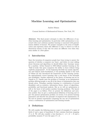
function. This function is nevertheless non-differentiable and non-convexand is thus not easy to minimize. In fact this problem is NP-hard so it ispointless to try to minimize this function. To deal with this problem weintroduce the hinge loss or margin loss given by φ(y, y 0 ) max(0, 1 yy 0 )this function is an upper bound to the 0 1 loss as shown in the figure,it is also convex and it turns out that [1]:minh measurableE(L(h(x), y)] minh measurableE(φ(h(x), y)which is indeed a desirable property. Thus we can replace the minimization problem by that ofminmax(0, 1 h(xi )yi )i 13.0h HnX1.50.00.51.0pmax(0, 1 - x)2.02.5Hinge loss0-1 loss-2-1012xFig. 1. Hinge loss is an upper bound for the 0 1 lossNow suppose the hypotheses class is given by linear functions h(x) wT x b for (w, b) Rn 1 thus the problem becomes:minwnXi 1max(0, 1 yi (xTi w b))
Or by adding some slack variablesminwnXζii 1subject yi (xTi w b) ζi 1ζi 0This is an empirical risk minimization problem and it is a linear programso we can easily solve it using the simplex method. Nevertheless we saidthat we needed to take into account the complexity of the hypothesesclass in particular we want to make the Rademachercomplexity small but for vectors in Rd that term is on the order of d 1 so if the dimensionis really big we might risk over-fitting data. This is known as the curseof dimensionality. A way of controlling the complexity is by boundingthe norm of the vector w as it was seen in example 3, so if we constrainkwk2 Λ we get:minwnXζii 1subject yi (xTi w b) ζi 1ζi 0kwk2 ΛWe can introduce a Lagrange multiplier λ 0 for the last constrain andobtainnXminwζi λkwk2 λΛi 1subject yi (xTi w b) ζi 1ζi 0Now here we assumed that we knew the optimal Lagrange multiplier forthe problem which is of course not true, but since we also don’t knowwhat is the best Λ we can just leave the problem asminwnXζi λkwk2i 1subject yi (xTi w b) ζi 1ζi 0and this is the support vector machine (SVM) optimization problem. Inpractice the parameter λ is tuned using cross-validation on a held-outdata set and that is what we did on this project.
4.2Ridge RegressionIf the loss function is the square loss then the natural optimization problem becomesminw,bnX((wT xi b) yi )2 .i 1Using a similar line of thought as in SVM we realize that if we wantto control the complexity of the hypothesis space we need to boundthe norm of w and so as before the optimization gets a ’regularization’parameter.min λkwk2 w,bnX((wT xi b) yi )2 .i 1This algorithm is known as ridge regression. The regularization parameter λ controls over-fitting of outliers as seen in the picture below.301020y4050lambda 0lambda 16lambda 322.02.53.03.54.04.55.05.5X[, 1]Fig. 2. Linear models for different values of λ. When λ 0 the slope is over slantedas it tries to fit the outlier as much as possible.
4.3AdaboostBoosting is a way of combining simple hypotheses to create more complicated ones what it does is the following: at every iteration t it keeps adistribution Dt over the training data, it picks the best classifier ht Hand picks a weight αt for this classifier, it then updates the distributionDt 1 by weighting more those points that wereP misclassified by ht andafter T rounds it returns the classifier hT ni 1 αt ht . The algorithmis completely described below:Algorithm 1 Adaboost pseudocodeRequire: (xi , yi )ni 1D1 (xi ) 1/nfor i 1 T doFind ht argminh H Di (h(x) 6 y) t Di (ht (x) 6 y)tαt 12 log 1 tDt 1 (xi ) Dt (xi )eend forPreturn Tt 1 αt ht αt yi ht (xi )Zt402exp(-x)6exp loss0-1 loss-2-1012xFig. 3. The exponential loss is an upper bound for the 0 1 loss.
The term Zt appearing on the algorithm is simply a normalization factor.We now see how to cast Adaboost as an optimization problem. Considerthe loss function L(h(x), y) exp( h(x)y) which is an upper bound forthe 0 1 loss as shown in the figure above. In [2] it is shown Adaboost isdoing coordinate descent on the loss function just described where everyiteration t is a step towards reducing the objective function. Although theprove of this is not hard it is rather long and is omitted, the interestedreader can find the proof in [5]. Intuition tells us that we should letour algorithm iterate as much as possible nevertheless this might leadto overfitting (although not always), in practice what’s done is earlystopping which means to stop the iterations before achieving a minimum,in this way we try to control the complexity of the hypothesis we arecreating. Other common practice to avoid overfitting is L1 regularization,i.e. minimizing the function:!nTXXexp αt ht (xi )yi kak1i 1t 1In the experiments we present the standard Adaboost and analyze it’sgeneralization ability.55.1ExperimentsClassificationFor the problem of classification we consider the data set of Arrhythmiafrom the UCI repository )the data set consists of 452 instances with 279 attributes, we used 352for training and 100 for testing. We present two different results.Oneis obtained by using empirical risk minimization of the hingeloss. Sincethis is a linear program we used the simplex algorithm to find the bestlinear classifier, as it can be seen in the plot for different training sizesthe training accuracy was always 1. Nevertheless the testing accuracywasn’t as good as the one given by SVM. For SVM since the data setwas really small we did cross validation to tune the parameter λ onlyfor the smallest training size (58) and then left that value of λ 16for the rest of the training sizes. As you can see the algorithm is reallylearning since the accuracy keeps steadily increasing as the training sizeincreases as opposed to empirical risk minimization where the testing error varies wildly from training size to training size. Another thing worthnoticing is that the training error is not as good as that of empirical riskminimization, this should be clear since SVM doesn’t optimize this butthe training and testing error seem to be converging as predicted by thebound (1)The following experiment shows the use of Adaboost in the same data,as our base classifiers we used stump functions: for every coordinatei {1, . . . , 279} we defineS a set of hypotheses Hi {h R h(x) 1 if xi h} and H i Hi . Since the amount of data wasn’t hugewe let Adaboost run for 8 iterations and reported the results, after 4iterations of Adaboost the testing error is already at its minimum and
0100150200250300350Training sampleFig. 4. Accuracy of empirical risk minimization and SVM. Reg-train and reg-test represent the accuracy of the regularized algorithm (SVM)afterwards it starts to increase while the training error keeps decreasing,this is the overfitting effect that I described in the previous section andthe reason why early stopping is necessary as a regularization technique.0.50Adaboost training and test rationsFig. 5. Adaboost training and testing error
5.2Regression0.030We present the results on two different regression tasks. Both fromthe UCI repository, the first one is the communities and crime ities and Crime) thatconsists of 1994 points with 278 attributes each; we used 1800 for training and 194 for testing. As in the case of classification the λ parameterwas tuned by cross validation on the smallest training sample (400) andleft fixed to λ 6. We plot the error of the hypotheses against the training sample size, the greatest advantage of ridge regression over simpleregression is seen when the sample size is small where the error is 20%smaller the other plot shown is the square norm of the linear hypothesis w, big values on the norm of w mean that the vector was trying toexplain the training data as good as possible, i.e it was overfitting.NormReg-norm600.015240.020AccuracyNorm of 00140016001800400600800Training sample10001200Sample sizea)b)Table 1. Communities data. a)Accuracy of the regularized and unregularized versionof regression. b) Norm square of the vector wThe second data set is from the Insurance Company Benchmark whichis a classification problem in reality but can still be seen as a regressionproblem, the size of the data set was of 9000 points with 86 attributes,after cleaning the data we were left with 5500 points for training and1000 points for testing. In this particular challenge we can appreciatereally well the advantages of regularization, the labels of the data weremostly 0 with maybe less than 10% of them being one, while the nonregularized regression tried to adapt to this labels, the regularized versiontreats them more as outliers and focuses on getting the 0 labels correctlyas it can be seen in the norm plots where the regularized algorithm givesvectors with norms really close to 0 and the unregularized version isabove 50 and it takes the algorithm to see 1000 points to realize thatthose points are outliers.140016001800
50NormReg-norm3000.0501020Norm of estReg-train2000300040005000400600800Training sample10001200Sample sizea)b)Table 2. Insurance Company Benchmark. a)Accuracy of the regularized and unregularized version of regression. b) Norm square of the vector w6Implementations and softwareA note on the implementation of the algorithms. SVM training and testing was done with the lib-svm [3] library. The empirical risk minimizationwas done using the simplex method. Since the data set wasn’t too big Iused the implementation I had in my previous homeworks. Neverthelessfor the biggest training set the algorithm was too slow and I ended upusing the R implementation of the simplex method. The training of Adaboost was done in the whole training set, the implementation was donein R from scratch. Regression and ridge regression being unconstrainedquadratic programs had a close form solution that was calculated exactly. Nevertheless in regular regression when the amount of data wastoo little compared to the dimensionality; positive semidefinite Hessianswere obtained, in order to be able to deal with these problems we added10 4 I to the Hessian to make the problem strictly convex.140016001800
7ConclusionsThe role of optimization in machine learning is crucial and it is alwaysnecessary, in fact without the developments on quadratic programmingalgorithms like SVM and ridge regression wouldn’t be used in practicebecause of the size of the training samples. Nevertheless the use of rawoptimization without the aid of statistics can lead to serious mistakesin experimental design as we showed in the experiments presented inthis project. Although the problems treated here were of a modest size Ibelieve that they still exemplify in a real way the problem of overfittingand how to control the problem with the use of regularization and earlystopping. For really big data sets algorithms like SVM are no longeruseful since training on millions or billions of points becomes infeasible,so people have turned to online learning which was something I wantedto treat on my project but the lack of time didn’t allow me to.
References1. Peter L. Bartlett, Michael I. Jordan, and Jon D. McAuliffe. Convexity,classification, and risk bounds. Technical report, JOURNAL OF THEAMERICAN STATISTICAL ASSOCIATION, 2003.2. Leo Breiman. Prediction games and arcing algorithms, 1997.3. Chih-Chung Chang and Chih-Jen Lin. LIBSVM: A library forsupport vector machines. ACM Transactions on Intelligent Systems and Technology, 2:27:1–27:27, 2011. Software available athttp://www.csie.ntu.edu.tw/ cjlin/libsvm.4. Vladimir Koltchinskii. Rademacher penalties and structural risk minimization, 1999.5. Mehryar Mohri, Afshin Rostamizadeh, and Ameet Talwalkar. Foundations of Machine Learning. MIT Press, 2012.6. L. G. Valiant.A theory of the learnable.Commun. ACM,27(11):1134–1142, November 1984.7. Vladimir N. Vapnik. Statistical Learning Theory. Wiley-Interscience,1998.
Machine Learning and Optimization Andres Munoz Courant Institute of Mathematical Sciences, New York, NY. Abstract. This nal project attempts to show the di erences of ma-chine learning and optimization. In particular while optimization is con-cerned with exact solutions machine learning