WIXLIB

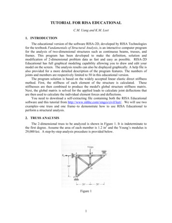
TUTORIAL FOR RISA EDUCATIONALC.M. Uang and K.M. Leet1. INTRODUCTIONThe educational version of the software RISA-2D, developed by RISA Technologiesfor the textbook Fundamentals of Structural Analysis, is an interactive computer programfor the analysis of two-dimensional structures such as continuous beams, trusses, andframes. This program has been developed to make the definition, solution andmodification of 2-dimensional problem data as fast and easy as possible. RISA-2DEducational has full graphical modeling capability allowing you to draw and edit yourmodel on the screen. The analysis results can also be displayed graphically. A help file isalso provided for a more detailed description of the program features. The numbers ofjoints and members are respectively limited to 50 in this educational version.The program solution is based on the widely accepted linear elastic direct stiffnessmethod. First, the stiffness of each element of the structure is calculated. Thesestiffnesses are then combined to produce the model's global structure stiffness matrix.Next, the global matrix is solved for the applied loads to calculate joint deflections thatare then used to calculate the individual element forces and deflections.You need to download a self-extracting file containing both the RISA Educationalsoftware and this tutorial from http://www.mhhe.com//engcs/civil/leet/. We will use twoexamples one truss and one frame to demonstrate how to use RISA Educational toperform a structural analysis.2. TRUSS ANALYSISThe 2-dimensional truss to be analyzed is shown in Figure 1. It is indeterminate tothe first degree. Assume the area of each member is 1.2 in2 and the Young’s modulus is29,000 ksi. A step-by-step analysis procedure is provided below.Figure 11

(1) Start the RISA-2D Educational program. Figure 2 shows that a manual bar willappear at the top of the window. In addition to a Data Entry toolbar, a global XYcoordinate system and a set of grid lines in the Model View window will alsoappear.manualbarFigure 2(2) If you have created an input file previously, click File from the manual bar andselect Open to open the input file. Otherwise, you can go to the next step to create anew model.(3) Click Global from the manual bar and enter the information for Model Title andDesigner in the Global Parameters window (see Figure 3). The program canprovide internal forces (moment, shear, axial force) at a number of equally spacedsections along a member. The default number of sections is 5, which is useful whenyou analyze continuous beams or frames. For truss analysis, however, the onlyinternal member force is axial load, and the axial load is constant along a trussmember. Set the Number of Sections to 2 so that the internal forces at both endsof the member will be provided. Click OK once you have completed theinformation.2

Figure 3(4) Click Units from the manual bar. One option you can choose in the UnitsSelection window is Use CONSISTENT units. This is the method we usually usefor hand calculations. That is, all the physical quantities like length, sectionproperties (A and I), material properties (E), loads, reactions, member forces, anddeformations are expressed in terms of consistent units (e.g., kips and inches). Forpractical applications, the program provides a more convenient way of handling unitconversions internally by allowing the designer to choose either the StandardImperial or Standard Metric units. We choose Standard Imperial in this example.Clock OK once you have selected the units.Figure 43

(5) Click Modify from the manual bar and select Grid. A Define Drawing Gridwindow will show that the program assigns, by default, (0, 0) as the coordinates forthe origin (see Figure 5). Furthermore, the program assigns 30 grids with a unitlength (1 ft) as the increment in each direction (see Figure 2). Considering theoverall dimensions of the structure in Figure 1, we can change the default setting to4@10 ft and 6@5 ft in the X and Y directions, respectively, such that all joints willfall on the grid. Save the Grid Settings and provide a description (e.g., DrawingGrid 1) for this drawing grid. If you open an existing file, it is necessary to Retrievethis grid settings in order to show the grids you previously defined. Click OK tocomplete this step. You will see the new drawing grid (see Figure 11).Figure 5(6) The next step is to provide data for the structure. If the Data Entry toolbar in Figure2 disappears for some reason, click Spreadsheet from the manual bar and selectData Entry Buttons Toolbar to activate it (see Figure 6).4

Figure 6(7) Click Joint Coordinates from the Data Entry toolbar to define each joint and itscoordinates. (Step 14 shows a more convenient way to specify joint coordinatesgraphically.) Follow the instruction in the Joint Coordinates window to defineeach joint (see Figure 7). The program by default labels each joint sequentially asN1, N2, . . ., etc. But you can rename each joint, as long as the joint name does notstart with a number (e.g., 1N). Click Edit from the manual bar or right click themouse and select Insert Line to add additional joints. Upon completing the jointdata, you can click View from the manual bar and select Joint Labels to check thejoint input graphically (see Figure 11).Figure 7(8) Click Boundary Conditions from the Data Entry toolbar to specify the supportcondition. For this example, joint A is supported by a vertical roller. Click the fieldfor X for a red arrow. Clicking on the arrow will allow you to define whether thatdirection is free to move, fixed, or supported by a spring. We specify joint A asFixed because it cannot move in the horizontal (or X) direction. Click Edit from themanual bar and select Insert Line to add another two entries for the supportcondition for joints C and E (see Figure 8). Clicking View from the manual bar andselecting , the program will show graphically the boundary condition of thestructure (see Figure 11). A horizontal green line at joint A means that the jointcannot move in the horizontal direction.5

Figure 8(9) Member information is provided in this step. A total of 7 truss members exist in thestructure. Click Members in the Data Entry toolbar to specify member data, whichinclude the member label, joint labels at both ends (I for near joint and J for farjoint), area, and Young’s modulus (see Figure 9). You can ignore the field ofmoment of inertia by using the default value because it is not needed for trussanalysis. The length of each member will be computed by the computer programautomatically. Since members in a truss are pin-connected at both ends, it isnecessary to “release” the moment at both ends of the member (that is, zero momentat member ends). This can be achieved by clicking the field of I Release (and JRelease). Clicking on the red arrow will then bring up the Set Member ReleaseCodes window (see Figure 9), from which you can specify that both ends arePinned. In the Model View window, the program will insert an open circle near themember end to indicate that moment has been released (see Figure 11). Also seeStep 14 for graphic input of members.6

Figure 9(10) Joint loads are specified in this step. Only a 9-kip vertical load is applied at joint B.Click Joint Loads from the Data Entry toolbar. Specify the joint label in the firstcolumn of the Joint Loads and Enforced Displacements spreadsheet (see Figure10). Specify L (Load) in the second column. The direction of load, which is in theY direction for vertical load, is specified in the third column. The magnitude of thevertical load is specified in the fourth column. Because the vertical load acts in thedownward direction, which is in the negative Y direction, the magnitude of the jointload is –9. [You can specify D (Displacement) in the second column for problemsthat involve support settlements.] Also see Step 14 for graphic input of loads.Figure 10(11) The last two entries (Point Loads and Distributed Loads) in the Data Entrytoolbar are used to specify loads that act on a member. These two entries are notneeded in this example because the truss, by definition, can only carry joint loads.The data entry is now complete. You can check the geometry, the boundarycondition, as well as the labels of joints and members graphically by clicking Viewfrom the manual bar. From the View drop-down manual, you can select whateverinformation including the applied load for display (see Figure 11).7

Figure 11(12) Now click Solve (or click theicon) from the manual bar. The program willperform the structural analysis. A Results toolbar will appear if the analysis issuccessful (see Figure 12). (Clicking Results from the manual bar and selectResults Button Toolbar can also activate this toolbar.) If the data entry isincomplete or the structure is unstable, the program will issue an error message. AJoint Reactions spreadsheet summarizing all the reaction forces will also appear inthe window. The last row represents the summation of all reaction forces in the Xand Y directions, respectively, which can be used to check global equilibrium.Figure 12 shows that the sum of horizontal reactions is equal to zero. In the verticaldirection, the summation of the vertical reaction forces (9 kips) is also inequilibrium with the downward external load (-9 kips).8

Figure 12(13) The joint deflection information can be viewed by clicking Joint Deflections fromthe Results toolbar (see Figure 13). Clicking Member Forces from the Resultstoolbar gives a summary of internal forces in all members (see Figure 14). Theseare the member forces calculated along each member. The number of sections forwhich forces are reported is controlled by the Number of Sections specified in theGlobal Parameter window (see Figure 3). The number of member segments is theNumber of Sections minus 1. The length of each segment is the same. Forexample, if you specify 5 sections, the member is divided into 4 equal pieces, andthe forces are reported for each piece (see Figure 15). As for the sign convention,the signs of these results correspond to the member's local axes, using the right handrule. The left side forces at each section location are displayed. There are threeforce values for each section location. These are axial, shear and moment. As canbe seen in Figure 15, the section forces listed at any given section are the left sideforces. For axial forces, compressive is positive. For moments, counter-clockwisearound the member axis is positive.9

Figure 13Figure 14Figure 1510

(14) Note that creating the model and specifying loading as described in step (6) throughstep (11) can also be performed graphically. Figure 16 shows the icons that can beused for this purpose. For example, clicking the third icon () allows you tospecify both the joints and members. The support conditions can be specified byclicking, and the loadings can be specified by clicking either one of.graphic input iconsFigure 1611