Transcription
ReportVisualisation of User Defined Finite Elements with ABAQUS/ViewerVisualisation of User Defined Finite Elements withABAQUS/ViewerS. Roth, G. Hütter, U. Mühlich, B. Nassauer, L. Zybell, M. KunaInstitute of Mechanics and Fluid Dynamics, TU Bergakademie FreibergAbstractCommercial finite element (FE)software packages provide interfaces for user defined subroutines, e.g. to define a user definedmaterial behaviour or special purpose finite elements, respectively. Regarding the latter, themajor drawback of user definedelements in Abaqus is that theycan not be visualised with thestandard post-processing toolAbaqus/Viewer. The reason forthis is that the element topology is hidden inside the elementsubroutine.The software tool presentedwithin this contribution closesthis gap in order to utilise thepowerful Abaqus postprocessingpotentials. Because only elementsfrom the Abaqus element librarycan be visualised with Abaqus/Viewer, the user elements inthe output data bases resultingfrom FE calculations are replacedwith properly chosen elementsfrom the Abaqus standard element library. Furthermore, userelement related data are takenfrom the binary results files andtransferred consistently to thesestandard elements. This is doneby means of the Abaqus Pythonscripting interface and requiresthe provision of additional userdefined information concerningthe element topology.The capabilities of this softwaretool are demonstrated with userdefined elements developed fornon-local damage mechanics,gradient elasticity, cohesive zonemodels and ferroelectricity.1. IntroductionFinite element (FE) solutionschemes require in general asummer 2012rather complex overhead including the pre-processing, properdata organisation etc. In addition, sophisticated solvers, contact algorithms or other toolsare involved. Furthermore, theamount of manpower and timeneeded for the maintenance ofsuch complex software solutions should not be underestimated.The user element interface provided by the commercial FE program Abaqus enables researchesworking in different fields ofcontinuum mechanics, to focusexclusively on their specific problems without being forced totake care of the topics mentionedabove. Unfortunately, Abaquscan only visualise built-in elements with the correspondingpost-processing tool, Abaqus/Viewer. However, Abaqus provides tools to extract information from output database files.The latter contain all requesteddata of the FE analysis includingmodel information and results.The particular structure of thesefiles relies on the Abaqus dataconvention which is documented in the corresponding manuals[1]. Therefore, all the necessaryinformation can be extracted, enriched and re-structured in orderto use the outcome of this process for the Abaqus/Viewer. Theuse of another post-processingsoftware would be possible too,but there are certain objectionsconcerning this idea. First of all,it is rather unlikely that alternative visualisation tools provide all the specific facilities supported by the Abaqus/Viewer.The simultaneous use of varioustools according to their parti-cular advantages is not seenas a suitable alternative either. Second, independent of theparticular choice, data conversion has to be performed always.This means that the use of otherpost-processing tools than theAbaqus/Viewer would not provide any benefit regarding thedevelopment cycle of the software necessary to achieve thedesired objective.A particular strategy for thevisualisation of user elements issketched already in the Abaqusmanuals. However, this strategyhas several serious drawbacks.Here, a solution is proposed thatresolves these problems.The paper is organised as follows.First, the Abaqus data structure is examined in order to derive the minimum requirementsfor a suitable visualisation strategy. Subsequently, different possibilities to accomplish the taskare outlined and the particularadvantages and disadvantagesare discussed, focusing especially on the solution proposedhere. Afterwards, the latter isdescribed in more detail andits capabilities are demonstratedby means of several illustrativeexamples.2. Visualisation strategiesPlotting of user elements isnot supported in Abaqus/CAE [1]. The Abaqus/Vieweronly supports the visualisation of built-in elements of theAbaqus element library, whichare hereinafter referred to asstandard elements. There isno interface to specify user defined elements in the viewer.This leads to the questions what7
Visualisation of User Defined Finite Elements with ABAQUS/Viewertype of interface would be necessary to overcome this and whichelement data should be transferred? For visualisation purpose, theviewer requires the topologicaldata of the finite elements. In thiscontext, element topology coversthe number of nodes and thedefinition of vertices, edges andfaces which specifies the nodesmutual positions. Furthermore,in order to plot integration pointdata like stresses or state variables,the number of the integrationpoints as well as their positioninside the element are of interest.Finally, the shape functions define an inter- and extrapolationalgorithm to determine the integration point values out of nodaldata and vice versa, respectively.Of course, all this informationis enclosed in the user elementsubroutine. But outside, onlythe number of nodes, the nodaldegree of freedom (DOF) andthe amount of memory requirements for internal state variablesare known. This suffices for theFE solution procedure but notfor visualisation. Here, it shouldbe emphasised, that these problems are not only limited tothe Abaqus framework. Pre- andpost-processing of ANSYS userelements, for instance, is boundto the specification of a so-calledkeyshape value determining theelements topology [2].However, in order to use Abaqus/Viewer to visualise user elementsin spite of all, additional effortis unavoidable. Thus, alternativestandard elements, in the following called dummy elements, arechosen from the Abaqus elementlibrary and displayed in place ofthe user elements. Therefore, thetopology of the dummy elementsand the user elements shouldbe as similar as possible. Thisconcerns the element shape (e.g.hex, wedge or tet in 3D), thenumber of nodes, the order of theshape functions and the numeri8cal integration (number and position of integration points). It ispart of the developers job to finda balance between the restrictionsconcerning functionality of theuser element and its visualisationability with the help of an applicable dummy element. Mostly, acompromise is found since theelement library provides a largevariety of standard elements.The next step towards a successfulvisualisation is the extraction ofthe nodal and integration pointresult data from a data base.Therefore, the internal data structure of the output database file(odb) is considered, wherein fieldoutput is assigned according toa so-called field location whichspecifies the position for whichfield data are available (e.g. node,integration point) [1]. Regardinguser elements, the informationabout the field location and integration points is hidden insidethe element subroutine and thusthe assignment of user elementrelated result data fails. For thisreason, user element output iswritten to either results file (fil)or data file (dat) while nodal fieldvariables can be written to odb, filor dat. A further important aspectconcerns the interpretation ofthe element output. The arrayof solution dependent variables(SDV) is composed by the userelement subroutine and can besplit into several integration pointrelated SDV arrays. A decomposition of them into field quantitiesrequires additional informationabout their name, descriptionand tensorial rank. The latter isnecessary to allow Abaqus to provide the tensor invariants.In summary, a visualisation interface has to manage1. the input of additional elementdata concerning element toplogy,the desired dummy element andSDV arrangement,2. the generation of the dummyelement mesh,Report3. the transfer of nodal data andSDV to the odb, and4. the two-step decompositionof the SDV array with respect tothe number of integration pointsand the embedded field quantities.There are a couple of approaches within the Abaqus framework discussed in the following.Afterwards, the favoured one isdescribed in more detail.2.1. State of the artIn order to visualise the shapeof user elements, the AbaqusAnalysis User’s Manual [1] proposes an overlaid mesh of standardelements generated during thepre-processing. In combinationwith an almost vanishing material stiffness associated, the overlaiddummy element mesh allows thevisualisation of the deformationstate [1]. The spurious influenceof the dummy element meshon the numerical result is eliminated if an additional dummyuser material is defined just creating zero stiffness matrices [3].Furthermore, the definition ofthe dummy elements with thehelp of the existing nodes ofthe user element mesh allowsfor visualisation of all nodal fieldquantities, e.g. displacements,nodal temperatures and reactionforces. Regarding the computational cost, the additional effort islimited then to the evaluation ofthe dummy material subroutines.The size of the system matrices ofthe finite element models is notaffected as neither the number ofnodes nor the nodal DOF changes. The latter requires a compatibility between the nodal DOF ofthe user element and the dummyelement which limits the choiceof possible dummy elements.Concerning the transfer of element output, it is recommendedto use the subroutine UVARM,which is called at the end ofevery increment at every integration point of the dummy elementsummer 2012
Reportmesh to generate element output.The exchange of data between theUVARM subroutine and the corresponding user element subroutine is usually managed via common blocks, i.e. shared memory,or modules. Unfortunately, theuse of common blocks is explicitly precluded for multiprocessingapplications [1] which gives riseto the major drawback of thedata transfer via UVARM. Therenouncement of efficient computational performance, i.e. parallel computing, for the benefit ofvisualisation seems to be a poorcompromise especially regardingthe simulation of large models.Furthermore, in order to interpret the element output, subsequent post-processing remainsindispensable since the UVARMjust passes the still unstructuredSDV array of the respective integration points. Last, the increaseof computational time due tothe dummy element operationsis considerable, depending on thenumber of user and dummy elements, respectively.Thus, it can be stated that thestrategy presented does not meetall the requirements of a visualisation interface mentionedabove. In particular, the limitinginteraction with the numericalcomputation is hardly acceptable.Instead, an independent visualisation module, applicable to arbitrary user elements should beenvisaged.2.2. Postprocessing visualisationstrategyThe visualisation strategy proposed here, called hereafterAbaquser, is a post-processingapproach. In contrast to the strategy described before, the FE calculations are not affected and there areno spurious enlargement of computational time or other restrictions to be met. Abaquser baseson the Abaqus Python scriptinginterface which is used to addsummer 2012Visualisation of User Defined Finite Elements with ABAQUS/Viewermodel and result data to the odbafter extraction from fil. Moreover,decomposition and interpretationof the SDV array is performed,too. Before presenting this purepost-processing script package inmore detail and demonstrating itscapabilities, it should be mentioned that there is a third applicablealternative of visualising user elements. It comprises the combination of both strategies, i.e. thepre-processing generation of anoverlaid dummy element meshwith zero-stiffness user materialcombined with a post-processingtransfer of element data from fil toodb. Compared to pure post-processing, the latter strategy yieldsless post-processing costs sincethere is no need to transfer nodaldata. In return, the modelling ofthe overlaid mesh and the evaluation of the dummy elementsmaterial subroutine result in comparatively higher pre-processingand computational costs.3. AbaquserAbaquser, a collection of shelland Python scripts manages alloperations required to get anodb, which can be visualised withAbaqus/Viewer, for a given FEmodel containing user elements.It comprises four scopes explained in the following. A schematicdiagram of the working sequenceof Abaquser is depicted in Figure 1.3.1. Controlling the FE calculation and visualisation postprocessingAll relevant processes related tothe visualisation are controlledby a shell script, abaquser.sh.Since the objective includes aninput file check with respect to allindispensable conventions, thisinvolves the submission of theFE job, too. Its command syntaxresembles the syntax of the Abaquscommand abaqus [1] supplemented by an option to specify the information file containing all additional data required.After the FE calculation has beencompleted successfully, visualisation post-processing is initiatedimmediately.3.2. Extraction of model andresult data from data baseModel and result data can beextracted out of different datasources. Since the efficiency ofthe visualisation process and itsaccuracy is quite sensitive to thischoice, here, the potential sources are discussed briefly. Thereby,it is appropriate to distinguishbetween model and result data.Model data related to user elements are available in the inputfile, dat or fil. User elementsresult data can be written to dator fil. Although implementedeasily and used severalfold, theuse of the ASCII format dat (seeFigure 1:Visualisation process of Abaquser.9
Visualisation of User Defined Finite Elements with ABAQUS/Viewer10Reporte.g. [4]) is not a good choice as data element. In two data lines nodes is firstly used. A better perforbase, because writing to the dat rai- and integration points of user mance is expected with the helpses computational time significant- element and dummy element of the C interface. However,ly. Furthermore, in comparison to are assigned. Subsequently, Abaquser is adapted to the interthe binary fil, there are major sto- field variables are defined (key- faces to achieve an efficient datarage requirements and less reading word *SDV) specifying its name, transfer. With Abaqus versionspeed. Due to the fixed number description, tensorial rank and 6.10 upwards, in order to speedformat, the accuracy is limited. For the position of its coordinates in up the visualisation post-procesthese reasons, the binary fil, which, the SDV array. Similarly, nodal sing, the extraction of the resultincidentally, can be written, too, in field variables can be re-interpre- data from fil and the odb updateASCII format, is chosen to be the ted. Furthermore, the dimension can be carried out in parallel bypreferred data source. It should be of the model has to be defi- means of the multiprocessingmentioned, that to the author’s ned (keyword *DIM). An excerpt module of Python 2.6.knowledge, visualisation of resultdata taken from fil by means of**Abaqus/Viewer is not published*DIMso far. To access the results fileTHREE D**information, Abaqus provides a*UEL, TYPE U1, NUMIP 3, NUMSDV 90, NUMSDVPIP 30, ABADUMMY AC3D61 2 3 4 5 6well described Fortran interface [1]1 2 3 1 2 3which is, however, not used here.***SDV, UEL U1Unfortunately, the model data inS Stress TENSOR 3D FULL 1 2 3 4 5 6the fil are not organised in theDELTA Separation Vector VECTOR 7 8 9DAMAGE Scalar Damage Variable SCALAR 10assembly-instance structure which.**the Python interface expects toupdate the odb. Nevertheless, itFigure 2:2: Excerptofinformationthe informationfilefilerelatedrelated totoa 6-nodecohesivezone userelement,Section 4.3.is possible to re-build the desi- FigureExcerptof thea 6-nodecohesivezoneuserseeelement,red structure with the help of the see Section 4.3.respective node and element labels,Abaquseruses the data from the information file to re-arrange the user element definition got from fil with respewhich contain the assemblyas welltothedummyelement’snode ordering.Regarding fileresultisdata,reading examplesthe SDV fromthe unstructured arrayas the instance labels. This leads toof suchan information4.afterIllustrativeforfilappliare decomposed with respect to the formerly unknown number of integration points and to the specific field quantitiethe requirement that each of the shown in Figure 2.cationFurthermore, model and result data are sorted and grouped according to the Abaqus Python update interfaces in ordnodes and elements defined in the Abaquser uses the data fromto prepare the odb update best possible.pre-processing has to belong to at the information file to re-arran- 4.1. Non-local ductile damageleast one set whose3.4.labelis evaluOdbupdate ge the user element definition In the range of room temperaated later on. Otherwise, this entity got from fil with respect to the ture, typical engineering metalsThe Abaqus scripting interface [1] enables the creation of new odb and the update of existing ones. For reasoncan not be assignedoftosimplean instancedummytheelement’snodeis firstlyorde- used.likeAsteelby a ductilemecha-with the help of thimplementation,Python interfacebetterfailperformanceis expectedand its visualisationC fails.interface. However,ring. reAbaquser is adapted to the interfaces to achieve an efficient data transfer.With eparticversion 6.10 upwards, in order to speed up the visualisation post-processing, the extraction of the result data from fi3.3. Input and evaluationaddiarraysare decomlesthewhichbreak or moduledebondoffromand the ofodbupdateunstructuredcan be carried outin parallelby means ofmultiprocessingPython 2.6.tional user element information posed with respect to the for- the embedding metallic matrix.The visualisation processrequiresexamplesmerly forunknownnumber of inte- These voids grow and finally4. Illustrativeapplicationadditional information concer- gration points and to the specific coalesce. In the coalescence stageNon-localdamagening the dummy 4.1.elementsandductilefieldquantities. Furthermore, the deformation localises withinthe interpretation of Intheresultand result typicaldata aresor- onelayerof steelvoids.fail by a ductile mechanism. In ththe range ofmodelroom temperature,engineeringmetalslikedata, i.e. the SDVarray.voidsThisted andaccordingClassicaldamagelikethose metallic matriprocess,are k ordebondmodelsfrom theembeddingThese voidscoalesce.In updatethe coalescencedeformationlocalises withininformation is providedby growan andthefinallyAbaqusPythoninter- stageaftertheGursonor Rousselierintro-one layer of voids.damagemodelslike thoseafter Gursonor Rousselierthe voidvolumeadditional file, calledClassicalhereafterfacesin orderto preparethe odbduce the introducevoid volumefractionas fraction as oidgrowthadequately.However,thesemodelsinformation file, similarly struc- update best possible.further internal variable allowingpredict a chisnon-physicalandtheleadsto ofthevoidwell-knowntured to the Abaqus input file.to describestagegrowth pathological messensitivity*UEL)in FE-simulations.Element data (keyword3.4. Odb updateadequately. However, these modelsFor this reason, a non-local modification of the Gurson-model was developed [5]. In a so-called implicit gradiencontain the user element’s name, The Abaqus scripting interface predict a localisation zone of zeroenriched formulation a further partial differential equation is incorporated introducing an intrinsic length scale asthe number of integration points, [1] enables the creation of new width in the coalescence stagefurther material parameter. This intrinsic length can be correlated to the mean spacing of the voids and allowsthe number of SDV,the numberand the updateof existingwhichnon-physical and leads tocontrolthe width ofodbthe localisationzone of voidcoalescencein theissimulations.of SDV per thewell-knownmesh as additional sweak form of the further partial differential equation has to be includedpathologicalin the FE-formulationthe name of the sensitivityin FE-simulations.of equations.Correspondingly,non-local(the non-localvolumetricplastic strain) enters as nodal variablThe additional non-local equations are implemented as a user defined element via the UEL interface.Three-dimensional hexahedral as well as two-dimensional plain-strain and axisymmetric elements have been dsummer 2012veloped in a large displacement formulation for static or dynamic applications. Quadratic shape functions are usefor the geometry and the displacements and linear ones for the non-local volumetric plastic strain. Full or reduce
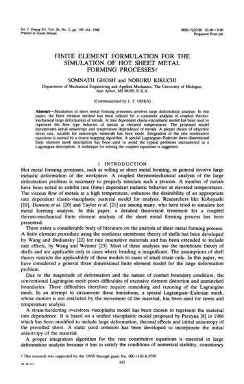
ReportVisualisation of User Defined Finite Elements with ABAQUS/ViewerFigure 3:Distribution of the void volume fraction after necking in a tensile test.Figure 4:Final damage state (porosity f ) obtained with regular finite element meshes using different element edge lengthsalong the path from the upper left corner to the lower right corner of the square (lhs). The contour plot of the damagevariable (rhs) corresponds to the simulation performed with the finest mesh 1/64. The ratio between the length ofthe square and the internal length R is 0.25, see e.g. [6]. An initial porosity f0 0.1 was used for all simulations and thefinal porosity fF was set to fF 0.95.For this reason, a non-local modification of the Gurson-modelwas developed [5]. In a so-calledimplicit gradientenriched formulation a further partial differentialequation is incorporated introducing an intrinsic length scale as afurther material parameter. Thisintrinsic length can be correlatedto the mean spacing of the voidsand allows to control the widthof the localisation zone of voidcoalescence in the simulations.The weak form of the further partial differential equation has tobe included in the FE-formulationas additional set of equations.Correspondingly, the non-localvariable (the non-local volumetric plastic strain) enters as nodalvariable. The additional non-localequations are implemented as auser defined element via the UELinterface.summer 2012Three-dimensional hexahedral aswell as two-dimensional plainstrain and axisymmetric elements have been developed in alarge displacement formulationfor static or dynamic applications. Quadratic shape functionsare used for the geometry and thedisplacements and linear ones forthe non-local volumetric plasticstrain. Full or reduced integrationis available. The Abaqus built-inelements CPE8, CPE8R, C3D20 orC3D20R are used as dummy elements for the visualisation withAbaquser. Figure 3 shows thedistribution of the void volumefraction in the late stage of thenecking in a tensile test simulated with the non-local Gursonimplementation in Abaqus.4.2. Quasi-brittle strain gradientdamageModels aiming to describe quasi-brittle failure must incorporate the evolution of damage.Furthermore, they should accountfor deterministic size effects andthe numerical results obtained bythese models must not show anyspurious mesh dependence. Basedon the constitutive equations forstrain gradient elasticity derived in[6] and [7] a continuum damagemodel has been developed. It restson the idea to describe the damageevolution in porous elastic materials by means of the evolution ofan effective porosity which canincrease beyond an initial value f0,related to the undamaged porousmaterial, up to a final porositysomewhere in between the initialvalue and one. The main ingredient of the damage model is a11
Visualisation of User Defined Finite Elements with ABAQUS/Viewerdamage surface which depends regular meshes varying the edgeon the macroscopic strains, its size of the finite elements fromspatial gradients and the effective 1/8 down to 1/64. Parts of theporosity f.results are shown in Figure 4.The appearance of strain gradients Because the visualisation toolor second gradients of the dis- enables the user to take advanplacements, respectively, requires tage of all features provided bythe use of either C(1)-continuous Abaqus/Viewer, like contourfinite elements or a suitable mixed plots, plots of variables along afinite element formulation. Here, path, etc., it is not just useful tothe latter was preferred using gether with the final user elementadditional Lagrange multipliers. solution but it is also extremeNevertheless, neither one of these ly helpful during the process oftwo options mentioned above implementation and testing.forms part of the current standard element library of Abaqus. 4.3. Fatigue crack growth ofTherefore,a userdefinedsolutiontribution of the void volumefraction afterneckingin a tensiletest. is thermally sprayed coatingsanyway. The damage The simulation of thermo-mechaction after necking in aunavoidable,tensile test.model has been implemented into nical fatigue of thermally spraymagethe FE program Abaqus extending ed coatings is performed withi-brittle failure mustthe evolutionof damage. theFurthermore,theincorporateuser elementalready describedhelp of theycohesive zone delsmustnot showany [9]. The coatingorporate the evolutionof damage.Furthermore,theyin [8].The ninenoded elementelements(CZE)n theconstitutivefor straingradientelasticityderived in [6] and [7] aalresultsobtainedequationsby these modelsnot showany atcontainstwo mustdisplacementsconsists of deformed, ageevolutionin porous elasticns for strain gradientelasticityderivedin [6] and [7]aallnodes,fouradditionalstrainsparticles, related by thin initialvaluef0separatedidea to describe the damage evolution in porous elasticatthecornernodesandfourlayers,wheredamage accumulap to a finalporosity beyondsomewherein betweeninitial value and one. The mainwhichcan increasean initialvalue thef0 , relatedLagrangemultipliersat Thethe mainmiddletionis supposeddamageinsurfacewhichdependson thestrains, itsspatialgradients to be situated.ewherebetweenthe initialvalueand entativevolume elementepends on the macroscopic strains, its spatial gradientsnts or second gradientsthe displacements,ofCPE8ofelementis used asrespectively,dummy requires(RVE ofthetheusecoatingstructure) issf atterwaspreferredthe displacements,respectively, requires the use ofelement.depicted in Figure 5. The partics. elementNevertheless,neitherone ofthethesetwooptionsmentionedforms part is obtained byteformulation.Here,latterwaspreferredThe convergencebehaviourofthe edsolutionisunavoidable,anyway.Theone of these two el hasVoronoi-tessellation taking intod, adydescribedinuser defined solution is unavoidable, anyway. Thebyat meansoffourtheadditionalfollowingproaccountthe meandiameter of thesbaqustwo tending the user element already described sed as dummy element.l nodes,additionalthestrainsat theCPE8cornernodes isandquadraticboundarydisplacementsles. Both, substrate and particlese standard CPE8 elementis usedas dummyelement.1 2and u2 0.05( x12 are) referring toto abe linear elastic.u1 0.05( 12 x12 x22 ) and2 x2assumed1 21 2 referring to a22Thetraction-separationrelation0.05( 2 x1 x2 ) and u2 0.05( x1 2 x2 ) referring to a//64.PartsoftheresultsCartesian coordinate system with at the interfaces between the coa/the origin /64.Partsupperof the resultsin theleft cor- ting particles and between coaner of the square. The simulati- ting and substrate are describedons were performed with different with a cyclic cohesive zone modelReportFigure 5:RVE of a thermally sprayed coatingstructure.[10]. Misfits of elastic modulusand thermal expansion coeffcientcause thermo-mechanical fatiguewhen the structure is subjected tocyclic thermal loading. Figure 6shows the distribution of damageat the honeycomb-like CZE meshafter various load cycles.The implemented CZE provideboth linear as well as quadratic shape functions, which arenot supported in Abaqus [1].Moreover, in contrast to Abaqusstandard cohesive elements truestress and strain tensors are available. In 3D stress/displacementanalyses with 12 node quadraticwedge-shaped CZE linear acoustic AC3D6 elements with higher order integration are usedas dummy elements. This choicesucceeds only using the pure postprocessing strategy. Otherwise,the overlay mesh of acoustic elements increases the nodal DOFwhich leads to an unnecessaryinflation of the system matrices 1/8 1/16 1/32 1/64 02ined with regular finite element meshes using different element edge lengths along the path fromr of the square (lhs). The contour plot of the damage variable (rhs) corresponds to the simulationmeshes using differentFigureelement6:edge lengths along the path fromhe ratio between the length of the square and the internal length R is 0.25, see e.g. [6]. An initialour plot of the damage Damagevariable (rhs) corresponds afterto the 4simulationand 9 thermal load cycles, cut view through RVE.and the final porosity fF was set to distributionf 0.95.he square and the internal length R Fis 0.25, see e.g. [6]. An initialto fF 0.95.126summer 2012
Reportand computational cost, respectively. The visualisation is mainlyfocused on the damage distribution and allows the quantificationof fatigue crack growth withinthe cohesive zone and decohes
ches within the Abaqus frame-work discussed in the following. Afterwards, the favoured one is described in more detail. 2.1. State of the art In order to visualise the shape of user elements, the Abaqus Analysis User's Manual [1] propo-ses an overlaid mesh of standard elements generated during the pre-processing. In combination