Transcription
High-performance Abaqus simulationsin soil mechanicsH.M. Hügel, S. Henke, S. KinzlerInstitute for Geotechnics and Construction Management, Hamburg University of Technology,GermanyAbstract: Abaqus is often applied to solve geomechanical boundary value problems. SeveralAbaqus built-in features enable a wide range of simulating such problems. For complex problemsAbaqus can be extended via user subroutines. Several extensions for soil mechanics purposes arediscussed and corresponding case studies are presented.Keywords: Abaqus, soil mechanics, soil plasticity, hypoplasticity, pile penetration analysis, soilcompaction analysis, quay wall deformation analysis, quay wall optimization analysis, Abaqusand MATLAB1. IntroductionBoundary value problems in soil mechanics are non-linear due to material non-linearity (always),geometrical non-linearity (sometimes) and non-linear boundary conditions for problems with soilstructure-interaction (often). They can imply complex construction processes like penetration ofstructures into subsoil causing propagation of waves in subsoil and actions on existing structures.Soils are modelled as single-, two- or three-phase materials depending on the existence andvolume fractions of soil constituents like soil particles, pore water and pore air. Correspondingmechanical models range from classical continuum mechanics up to theories of mixtures likeTheory of Porous Media. Moreover boundary value problems are commonly characterized by adisadvantageous ratio of characteristic lengths of the subsoil section to smallest dimension ofstructures, which makes three-dimensional models rather complex. Sophisticated computersimulations in soil mechanics need FE-formulations for finite deformations, contact algorithms forfinite relative motions and parallelization algorithms. Abaqus offers a wide range of built-infeatures for soil mechanics purposes and can be extended using several user subroutines.2. Abaqus built-in features for soil mechanics purposesA listing of Abaqus built-in features to solve boundary value problems in soil mechanics readswithout demand on completeness:2008 Abaqus Users’ Conference1
Several finite elements with displacement, pore water pressure, temperature andconcentration degrees of freedom can be used to discretize the soil body for one-, two- andthree-dimensional stress-deformation, seepage, heat transfer and diffusion problems. Constitutive models for soils: Mohr Coulomb plasticity (linear elastic, perfectly plasticmodel with Mohr-Coulomb yield condition and non-associated flow rule), extendedDrucker Prager plasticity models (linear or non-linear elastic, perfectly plastic or isotropichardening with alternative extended Drucker-Prager yield conditions), modified DruckerPrager/cap model (linear or non-linear elastic, volumetric hardening using cap surface,extended Drucker-Prager yield condition), clay plasticity (non-linear elastic, volumetrichardening model based on modified Cam Clay model). All these models are conservativeand do not contain modern concepts of soil modelling like for example double hardeningmodels, bounding surface plasticity or hypoplasticity. Time-depending linearly distributed Dirichlet and Neumann boundary conditions can bedefined for all active d.o.f. Linearly distributed initial values of effective stresses σ0, void ratio e0, pore pressure u0 ordegree of saturation Sr0 can be defined within element and node groups. Solution procedures: geostatic stress-displacement analysis for equilibrium iteration forinitial states, static stress-displacement analysis and dynamic stress-displacement analysisbased on implicit and explicit time integration for soils modelled as single-phase material,coupled consolidation analysis for soils modelled as two-phase materials (fully saturatedsoils), steady-state and transient thermal analysis for simulation of heat transfers in soilsdue to heat conduction and convection, steady state and transient diffusion analysis forsimulation of mass transport in soils. Load history: Typical actions like nodal forces, distributed forces or prescribeddisplacements can be defined. Excavation and fill of soil can be modelled by (de)activatingcorresponding finite elements in the model. Solution algorithms: Different algorithms to solve linear and non-linear systems ofequations are implemented. Soil-structure interaction problems can be solved applyingdifferent contact algorithms. ALE smoothing technique helps to stabilize the solution offinite strain problems.3. Abaqus extensions for soil mechanics purposesFor special purposes like new field equations, finite elements, constitutive or contact models aswell as coupling with external programs Abaqus can be extended via user subroutines.3.1 Field equations and finite elementsRegularization methods: Abaqus is based on classical continuum mechanics. In certain cases likesoil mechanical problems with large deformations and shear zone propagation the restrictions of22008 Abaqus Users’ Conference
this theory are tried to overcome with so-called regularization methods like Cosserat Continuum,Gradient Methods or Non-local Theories. Cosserat Continuum elements have additional rotationaldegrees of freedom. Implementations of corresponding two-dimensional elements in combinationwith hypoplastic constitutive models for soils were shown for example by Huang and Bauer(2001), Nübel (2002), Maier (2003) and Slominski (2007). Abaqus implementations forelastoplastic models can be found for example in Alsaleh (2004) and Arslan (2006). A comparisonof Cosserat Continuum, Gradient Method and Non-local Theory elements implemented in Abaquswas published by Maier (2003).Multi-phase dynamic analysis: The Abaqus built-in procedures do not cover multiphasedynamics, i.e. dynamic consolidation analysis for saturated or unsaturated soils is not possible.Nevertheless such procedures can be realized by implementing user elements with correspondingdegrees of freedom. In Holler (2006) an implementation of such a user element based on theTheory of Porous Media is shown for ANSYS. An implementation of his approach in Abaqus isunder work at our institute.3.2 Solution proceduresFully undrained analysis: Abaqus offers a fully coupled soil consolidation analysis. For certainreasons the fully undrained case is regarded, i.e. the whole FE domain is assumed to be undrained.This can be modelled in Abaqus/Standard in two ways: (1) a consolidation analysis with highloading velocity ensuring that the whole soil body is undrained, (2) a total stress analysis forexample with the Mohr Coulomb Plasticity formulated also in total stresses. Note that method (2)requires soil parameters for undrained conditions and is a fall-back on a material model being wellknown for poor prediction of deformations. In Abaqus/Explicit corresponding field equations andmaterial models can be implemented via user subroutines VUEL and VUMAT.Slope stability analysis: Besides stress-deformation analysis FEM can be applied to calculate thestability of slopes. This can be done for example with the Shear Reduction Method (SRM):beginning with an equilibrium state the shear parameters of soil are reduced step-by-step reachinga limit state. This is typically realized by reducing the shear parameters ϕ and c of the MohrCoulomb plasticity model. The factor of safety FS of the slope is than calculated using Fellenius'rule: FS tan ϕred/tan ϕext cred/cext (red reduced parameters, ext existing parameters.) Acorresponding solution procedure in Abaqus is not implemented. Nevertheless SRM can becarried out for example by defining temperature dependent shear parameters, an initialtemperature field. The SRM analysis is carried out by changing the temperature in a load stepcorresponding to a reduction of shear parameters.3.3 User defined constitutive models for soilsWith user subroutines UMAT and VUMAT user defined constitutive models can be implemented.They include the update of effective stresses σ (the apostrophe denoting effective stresses isomitted here for simplicity)i 1σi 1 σ&i h( , , ) d t σεσi t h(σ,σii 1, & , )εi2008 Abaqus Users’ Conference3
with a certain integration scheme approximating the integral (h is a tensorial function representingthe constitutive behaviour). In Abaqus/Standard the tangent operator C σ/ ε has to becalculated additionally. This can be done consistent to the chosen integration scheme to reachquadratic convergence of Newton’s Method or it can be approximated for example by numericaldifferentiation.Elastoplastic material models for soils should at least contain volumetric and deviatorichardening hypotheses in order to reach realistic modelling of soils (so-called double hardeningmodels). Linear elastic, perfectly plastic material models show many shortcomings, at least forprediction of deformations. The implementation of elastoplastic models in FE-codes is presentedin numerous publications dealing with computational plasticity. The implementation ofelastoplastic models in Abaqus is shown by Dunne and Petrinic (2005). Corresponding usersubroutines for elastic and elastoplastic models can be found underwww.eng.ox.ac.uk/solidmech/books/icp. User subroutines to implement certainelastoplastic models for soils can be found for example at www.soilmodels.info.Hypoplastic material models: Hypoplasticity is a completely different approach and is anextension of hypoelasticity: the Jaumann stress tensor (here denoted by a dot for simplicity) isformulated depending on rate of deformation tensor d and current state variables, e.g. effectivestresses σ and void ration e:σ& h( , d ,e )σThe tensorial function h is nonlinear with respect to d. Many hypoplastic models are decomposedin a linear (hypoelastic) and a non-linear part as follows:σ& h( ,d , e) L( , e) : d N ( , e) d σσσExisting hypoplastic models are able to describe a wide range of phenomena of mechanicalbehaviour of non-cohesive and cohesive soils (Gudehus, 1996; Niemunis and Herle, 1997;Niemunis, 2003). Applying the concept of intergranular strains (Niemunis and Herle, 1997) theycan be used to model cyclic and dynamic problems. The 4th-order tensor L and 2nd-order tensor Nare functions of state variables, typically effective stresses σ, void ratio e, intergranular strains δand overconsolidation ratio OCR. Hypoplastic models represents a set of 1st-order ordinarydifferential equations. It’s solution requires predefined initial conditions, here initial stresses σ0and initial void ratio e0. Implementing hypoplastic models in Abaqus is rather easy: inUMAT/VUMAT initial conditions for all state variables must be read at the beginning of analysis, theconstitutive equation(s) must be integrated and the tangent operator must be formulated. Thefollowing simple integration scheme can be used therefore:σi 1 t [( 1 )h(θ σiθσi, d ) h(σi 1, d )]For example θ 1 yields the well-known implicit Euler scheme:σi 14 t [L( σiσi 1) : d N(σi 1) d ]2008 Abaqus Users’ Conference
This represents a set of non-linear algebraic equations with the unknown stresses σi 1. It can besolved by linearization using (1) a predictor-corrector method, e.g. an explicit Euler step aspredictorσpi 1 σi t h(σi,d ) i 1 i 1,d ) 0σσi t h(σpi 1,d )(2) Newton’s Method to solve the non-linear equationr(σi 1) σi 1 σi t h(σ(3) Approximating the function h with truncated Taylor series:hi 1 hi h L: Li : σσσσ Ni N: σ σMethod (3) reads in index notation:i 1ijσ σiij Lijkl N ij Liijkl σ mn ε kl N iji σ mn ε pq ε pq σσmnmn Substituting σmn σijδimδjn we get σij Lijkl N ij Liijkl σ ij δ imδ jn ε kl N iji σ ijδ imδ jn ε pq ε pq σ mn σ mn Now σij can be extracted on the left side and the tangent operator can be build exactly, if thederivations L/ σ and N/ σ can be formulated analytically. User subroutines to implementcertain hypoplastic models for cohesive and non-cohesive soils can be found for example atwww.soilmodels.info and www.uibk.ac.at/geotechnik/res/khypo.html. Examplesbased on hypoplasticity are shown in Sections 4.1 to 4.4.3.4 User defined contact modelsAbaqus offers user subroutines UINTER and VUINTER to define normal and tangential behaviourof contacts as well as FRIC and VFRIC to implement friction models. Implementations forhypoplastic contact models based on user subroutine FRIC were shown by Gutjahr (2003) andArnold (2004).3.5 User defined boundary and initial conditionsNon-uniform boundary conditions of all d.o.f. can be defined via user subroutine DISP. They candepend on time, coordinates and element number. Non-linear distributed initial values of statevariables can be defined via user subroutines SIGINI for effective stresses σ0, with VOIDRI forvoid ratio e0 and with UPOREP for pore water pressure u0. If further state variables are introducedwithin user subroutine UMAT, the corresponding initial values can be defined with user subroutineSDVINI. All these user subroutines allow the definition of initial values depending on coordinates,element number for element variables and coordinates and node number for nodal variables.2008 Abaqus Users’ Conference5
3.6 Special modelling techniquesSimulation of penetration processes: One of the open questions of most geotechnical problemsis the simulation of the construction process which can cause relevant changes of state variables ofsoil, loading of already installed structures and a wave propagation in subsoil. The simulation ofprocesses like excavation and filling is standard in all FE-codes. Processes like boring, drilling,vibro-driving, quasi-static penetration and so on is non-standard but can be simulated in Abaqusunder certain conditions. For example the penetration of piles or other steel structures under quasistatic, harmonic or impact actions can be simulated using a kind of stripping technique: thestructure can penetrate into subsoil where a zipper was included into the subsoil before. Duringpenetration this zipper opens and allows to simulate the penetration without destroying the finiteelements. For axisymmetric problems this can be modelled with an interface between the soil bodyand a rigid line on the rotation axis. This technique was applied firstly in the 90's and wereextended at our institute to three-dimensional problems and structures with open cross-section tostudy the penetration of structures with arbitrary cross-sections into subsoil (Henke and Grabe,2006). An example is presented in Section 4.3.3.7 Coupling Abaqus with external programsFEM-BEM coupling: Limitations of infinite elements to model far fields of the solution domainare well-known. To overcome this shortcomings Abaqus can be coupled with Boundary ElementMethod, see for example Morra and Chatelain (2006). Hagen (2005) showed the coupling ofAbaqus with a self-written BEM-code. He programmed a user element enabling the iterativecoupling of a FEM sub-domain discretised by Abaqus and a BEM sub-domain discretised by aself-programmed time domain BEM program. The user subroutines UEL and UEXTERNALDB wereused therefore. The user element can be regarded as a superelement which includes all nodes ofthe interface between FEM and BEM sub-domains, but no internal nodes at all. Inside UEL thecoupling forces along the interface corresponding to the displacements of the coupled nodescomputed by Abaqus are calculated. They are handled as given boundary conditions for the BEMsub-domain. The BEM program is started inside UEL to calculate the interface forces for the giveninterface displacements. The BEM sub-domain contributes forces to the FEM sub-domain, butneither stiffness nor mass or damping contributions. User subroutine UEXTERNALDB is used topass information to the BEM program.Optimized design by coupling Abaqus and MATLAB: One main task in engineering design isthe determination of a system which fulfils best several requirements. Normally the blueprintprocess is conditioned by existing state of the art constructions and engineering experience.Wholistic approaches are missing which causes that a non-optimal solution is chosen. In order tooptimise geotechnical constructions we apply a coupling of Abaqus and MATLAB. MATLAB isa high-level technical computation language and interactive environment for numericalcomputation. In this language a non-linear multi-objective optimization algorithm based onevolutionary algorithms is coded and used for the optimization of standard laboratory test andseveral geotechnical design purposes such as sheet pile wall design (Kinzler and Grabe, 2006),spread or pile foundations (Kinzler, König and Grabe, 2007) so far. Abaqus is used to calculate themechanical response of the respective system, which is changed automatically from theoptimization algorithm. This result is viewed in common with others such as cost effectiveness or62008 Abaqus Users’ Conference
construction time and evaluated concerning the multi-objective optimization purposes. Themethodic change of Abaqus input parameters allows the location of the pareto-optimal set in astraight way. The case study in Section 4.4 shows an application.4. Case studiesThe following selected case studies are part of past and running research projects carried out at ourinstitute. For all simulations hypoplastic constitutive models for soils were applied.4.1 Simulation of soil compaction by vibratory rollers with Abaqus/ExplicitThe compaction of soils by vibratory rollers as shown in Figure 1 was studied using two- andthree-dimensional Abaqus models, see Kelm (2004) for a detailed description.Figure 1. Soil compaction by vibratory roller.The simulations were carried out for dry non-cohesive soils so that soil could be modelled as asingle-phase-material in uncoupled analyses. The anelastic soil behaviour is modelled usinghypoplastic constitutive models as mentioned in Section 3.3. In Figure 2 a three-dimensionalAbaqus model with 222600 elements is shown . The subsoil section is discretised using continuumelements (C3D8R) with displacement d.o.f. only, the far field is modelled with infinite elements(CIN3D8). The vibratory roller is simulated as a rigid surface linked with a point mass. Thehorizontal velocity and the vertical harmonic excitation of the roller is predefined. The dynamicstress-displacement analyses were carried out with Abaqus/Explicit.In Figure 3 the calculated distribution of void ratio e of soil is shown after a single vehiclecrossing. The vibratory roller leaves a zone of homogenized and compacted soil with a certaindepth depending on the machine parameters and initial state variables of soil. The Abaqussimulations helped us to optimise the compaction and homogenisation of non-cohesive soils. Moredetails can be found in Kelm (2004).2008 Abaqus Users’ Conference7
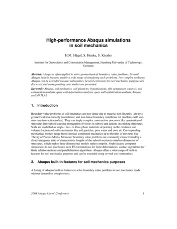
Figure 2. Abaqus model for simulation of soil compaction by vibratory roller.Figure 3. Calculated distribution of void ratio e after one vehicle crossing.4.2 Simulation of the deformation behaviour of a quay wall construction withAbaqus/StandardA class-A-prediction of the deformation of a quay wall construction at Hamburg harbour, seeFigure 4, was calculated using a three-dimensional Abaqus model (Mardfeldt, 2005). Theconstruction consists of a concrete plate, combined sheet pile wall, concrete piles and steelanchors. The 3D-Abaqus model shown in Figure 5 includes a three-dimensional section of thesubsoil and the superstructure for a section of 8 m of the quay wall. Using this model uncoupled(fully drained) analyses were carried out. The soil body, structures and soil-structure-interactionwas modelled as follows: C3D8R continuum elements (soil, concrete block, vertical concretepiles), S4 shell elements (inclined concrete piles, friction piles, combined sheet pile wall), overall129 contact pairs between structure and soil surfaces. The corresponding Abaqus model consistsof 111341 elements and 369735 d.o.f.82008 Abaqus Users’ Conference
Figure 4. Quay wall construction of Container Terminal Altenwerder, Hamburg.Figure 5. Abaqus model for deformation analysis of a quay wall construction.The material behaviour of structures was modelled with elastoplastic, the soil behaviour wasmodelled using hypoplastic constitutive models which were implemented via user subroutineUMAT as shown in Section 3.3. The highly non-linear character of the Abaqus model made the useof parallel computers necessary. 20 GByte of RAM were necessary for optimal Abaqusperformance therefore. The whole Abaqus/Standard 6.4 job took about 7 days of wall clock timeon a SMP architecure using 8 processors (the usage of more than 8 processors was not efficient2008 Abaqus Users’ Conference9
enough with this Abaqus version for this boundary value problem). The simulations allowed adeeper insight in the complex deformation behaviour of such a quay wall construction and helpedus to develop a design concept of steel anchors. For details see Mardfeldt (2005).4.3 Simulation of pile driving into subsoil with Abaqus/Standard andAbaqus/ExplicitA rigid pile is vibro-driven into subsoil as shown in Figure 6. Two- and three-dimensional Abaqusmodels are used to simulate the penetration process, the wave propagation in subsoil as well as theinfluence on existing piles in subsoil (Henke and Grabe, 2006; Henke and Hügel, 2007).Figure 6. Vibro-driving of piles into subsoil.To simulate the penetration of closed and open cylinders into homogeneous (layered) subsoilaxisymmetric Abaqus models are used. To simulate the penetration of cylinders in inhomogeneoussubsoils, of structures with open cross-sections and of structures in the neighbourhood of existingstructures three-dimensional Abaqus models are used. One of them is shown in Figure 7. Near andfar field of subsoil are modelled with continuum elements (C3D8R) and infinite elements (CIN3D8)respectively. The pile is discretized using a rigid surface. In Figure 7b a special technique topermit the penetration of the pile into the soil is shown: along the axis of penetration a rigid tubeof 1.0 mm radius is modelled. At the beginning of the analysis this tube is in frictionless contactwith the surrounding soil. During pile penetration the pile slides over the tube and the soilseparates from the tube so that contact between the penetrating pile and the surrounding soil canbe established. The main problem with such simulations is appearing mesh distortion caused bypile penetration, especially for wall friction angles larger than ϕ/3 of the soil. In axisymmetricmodels adaptive meshing based on ALE helps to overcome this problem. In three-dimensionalmodels adaptive meshing does not work so that the problem could be solved using a very finemesh in the neighbourhood of the piles only. Corresponding simulations have to run on parallelcomputers. Figure 8 shows determined speedup for Abaqus/Explicit 6.5 and 6.6 jobs running ontwo different SMP architectures. In these calculations one second of vibratory pile driving is102008 Abaqus Users’ Conference
modelled in a three-dimensional soil continuum consisting of 69401 finite elements, 78179 nodesand altogether 234543 d.o.f.’s, see Figure 7a. Almost optimal efficiency could be reached withAbaqus 6.6 with up to 16 processors using the domain level decomposition algorithm. The resultsconcerning the changes in the state variables of the surrounding soil can be found in Henke andGrabe (2006). This publication also discusses the effects of driving a pile in the center of anexisting pile group.Figure 7. Abaqus model for simulation of pile driving into subsoil.4.4 Optimization of a quay wall construction using Abaqus/Standard and MATLABA quay wall with a rather simple combined sheet pile wall is regarded as shown in Figure 9. Thedesign of such sheet pile wall constructions is a multi purpose optimization process. Clearlydefined requirements on the construction are faced with a plurality of possible varieties of staticsystems.Highly reduced, the construction process is composed of the determination of anchor- and sheetpile-profile as well as choice of the anchor inclination α and the grade of restraint provided by thesoil. The objectives are the tonnage of steel which is related to the total construction costs and thehorizontal deformation of the sheet pile head as a parameter for the serviceability of theconstruction. As a first step in the analysis the conventional verifications for a chosen set ofparameters are enforced. The tonnage results directly from the stress analysis in the ultimate limitstate.2008 Abaqus Users’ Conference11
Figure 8. Measured speedup for Abaqus jobs running on SMP architectures.Figure 9. Quay wall construction to be optimized.For a more realistic survey of the soil-structure interaction and the deformation behaviour thehorizontal deformation of the pile head is calculated by Abaqus. Therefore a parameterized, easymodifying model is generated. The model is separated into regions which are determined by dimensions chosen by the optimization algorithm. A regular mesh, controlled by a user specifiedglobal element size, is generated, see Figure 10. The intermediate steps of the construction processare modelled as well. All values depend on fractions of the constructive height of the quay wall. Inaddition to the dimensions the profiles are varied by choosing different material parameters for the122008 Abaqus Users’ Conference
anchor stiffness k and the moment of inertia I as well as the cross-section area A of the sheet pilewall. To allow a smart performance of the optimization, it is necessary to generate a mesh yieldingmoderate wall clock times. Former calculations indicate that a number of approximately 500nsimulations (where n is the number of objectives) seems to be sufficient. By analyzing automatically a multiplicity of various systems an effective optimization of the construction is the result ofthe analysis.Figure 10. Abaqus model for calculation of the horizontal deformation of the sheetpile head5 SummaryIt could be shown that Abaqus built-in features and Abaqus extensions based on user subroutinesand coupling with external programs can be applied to solve a wide range of boundary valueproblems in the field of soil mechanics. This offers researchers a tool to examine some of the openproblems in geomechanics like the influence of construction processes for geotechnicalconstructions, the optimization of geotechnical constructions regarding deformations or theoptimization of construction processes like penetration of structures into the subsoil. It should notbe concealed that the presented simulations have limits caused by modelling features andhardware resources. The need of future requirements on Abaqus features can be summarized asfollows: implementation of built-in sophisticated constitutive models for soils, improvednumerical stability for large deformation problems e.g. with modern ALE concepts and finallyenhanced efficiency in parallel computations as already shown in the last Abaqus revisions.2008 Abaqus Users’ Conference13
References1. Alsaleh, M., „Numerical modelling of strain localization in granular materials using CosseratTheory enhanced with microfabric properties. PhD thesis, Dep. of Civil and EnvironmentalEngineering, Louisiana State University, 2004.2. Arnold, M., „Zur Berechnung des Erd- und Auflastdrucks auf Winkelstützwände imGebrauchszustand“, Promotionsschrift, Mitteilungen des Instituts für Geotechnik derTechnischen Universität Dresden, Heft 13, 2004.3. Arslan, H., “Localization analysis of granular materials in Cosserat elastoplasticity –formulation and finite element implementation”, PhD thesis, Dept. of Civil, Environmentaland Architectural Engineering, University of Colorado, 2006.4. Dunne, F. and Petrinic, N., “Introduction to computational plasticity”, Oxford UniversityPress, 2005.5. Gudehus, G., „A comprehensive constitutive equation for granular materials”, Soils andFoundations, 31(1):1–126. Gutjahr, S., „Optimierte Berechnung von nicht gestützten Baugrubenwänden in Sand“,Promotionsschrift, Schriftenreihe des Lehrstuhls Baugrund-Grundbau der UniversitätDortmund, Heft 25, 2003.7. Hagen, C., “FEM-BEM coupling by means of Abaqus and user subroutines”. Internal report,Institute of Geotechnics and Construction Management, Hamburg University of Technology,2005.8. Helwany, S., “Applied soil mechanics with Abaqus applications”, John Wiley & Sons, 2007.9. Henke, S., Grabe, J., “Simulation of Pile Driving by Three-dimensional Finite Elementanalysis”, Proc. Of 17th European Young Geotechnical Engineering Conf., Zagreb, Crotia,ed. by V. Szavits-Nossan, Croatian Geotechnical Society, pp. 215 233, 2006.10. Henke, S., Hügel, H.M., „Räumliche Analysen zur quasi-statischen und dynamischenPenetration von Bauteilen in den Untergrund“. Tagungsband zur 19. deutschsprachigenAbaqus Benutzerkonferenz in Baden-Baden (Germany), 2007.11. Holler, S., „Dynamisches Mehrphasenmodell mit hypoplastischer Materialformulierung derFeststoffphase”, Promotionsschrift, Veröffentlichungen des Lehrstuhls für Baustatik undBaudynamik der RWTH Aachen, Heft 06/2, Wissenschaftsverlag, Aachen, 2006.12. Huang, W., Bauer, E., “A micropolar hypoplastic model for granular materials and its FEMimplementation”, Proc. of the 1st Asian-Pacific Congr. on Comp. Mech. (APCOM01), eds. S.Valliappan and N. Khalili, Sydney, Australia, Elsevier Science Ltd. press, 1135–1140, 2001.13. Kelm, M., „Numerische Simulation der Verdichtung kohäsionsloser Böden mitVibrationswalzen”, Promotionsschrift, Veröffentlichungen des Instituts für Geotechnik undBaubetrieb, TU Hamburg-Harburg, Heft 6, 2003.142008 Abaqus Users’ Conference
14. Kinzler, S.; König, F., Grabe, J., “Entwurf einer Pfahlgründung unter Anwendung derMehrkriterien-Optimierung”, Bauingenieur, 82(9): 367 379, 2007.15. Kinzler, S., Grabe, J., „Wirtschaftliche Optimierung rückverankerterSpundwandkonstruktionen”, Tagungsband zum Worksh
Abaqus built-in features enable a wide range of simulating such problems. For complex problems Abaqus can be extended via user subroutines. Several extensions for soil mechanics purposes are discussed and corresponding case studies are presented. Keywords: Abaqus, soil mechanics, soil plasticity, hypoplasticity, pile penetration analysis, soil