WIXLIB

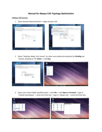
Manual for Abaqus CAE Topology OptimizationAbaqus CAE access:1. Open Exceed onDemand Client - login and pass 2FA2. Select “Desktop Mode Full Screen” (or other user preferred resolution) for XConfig and“Gnome Desktop.xs” for Xstart - click Run.3. Open user’s home folder (xyzXXX Home) - click File - click Open in Terminal - type in“module load abaqus” - press the Enter key - type in “abaqus cae” - press the Enter key.

4. Click with Standard/Explicit Model for general analysisAbaqus CAE basic:1. For official Abaqus CAE 6.14 User’s Guide, si/default.htm2. Interface

1. Main Manual: basic software function/support2. Model Toolbar: basic model functions and tools such as create/open/savemove/rotatequery information, zoom in/out, selection method, display options,,, etc.3. Model Tree: detailed information of model features and analysis output4. Module Manual: module/model/part selection5. Module Toolbar: module related tools (different from module to module)3. Unit system: Abaqus CAE has no inherent set of units. The user needs to decide which system ofunits to use. Some common systems of consistent units include:Abaqus CAE Topology Optimization:Before any analysis in Abaqus CAE, the user needs to create a new or open an existing model database(.cae file). A basic topology optimization process in Abaqus CAE involves 10 steps as shown:1. Create/import part(s) in the Part Module2. Assign material property to each part or part section(s) inthe Property Module3. Create instance and form an assembly ( 1 part) in the inthe Assembly Module4. Define analysis type, steps and outputs in the Step Module5. Add constraints/interactions between part-to-part and/orpart-to-datum in the Interaction Module6. Add loading(s) and boundary condition(s) in the LoadModule7. Generate FE mesh in the Mesh Module8. Define optimization type and parameters in theOptimization Module9. Create/manage optimization job(s) in the Job Module10. View/save results in the Visualization Module

1. Part Module1.1 3D part/assembly can be created directly in the Sketch Module of Abaqus CAE (NOTE:drawing CAD in Abaqus CAE is not recommended because it is not very user-friendly) orimported as STEP, SAT, IGES, etc. To upload CAD files onto hammer system, first send themonline (email or google drive), then use Firefox in hammer interface and download them(files will be automatically saved in the Download folder).1.2 Sometimes the imported geometry might have errors that Abaqus could not solve, then tryTool - Geometry Edit to fix them1.3 Use Tool - Partition to create subsections of a geometry (edge/face/cell). For example,select Cell type partition to divide a part into different volume sections for separatingdesign/non-design spaces and/or assigning different materials.

2. Property Module2.1 Create material(s): define Name and Material Behaviors (NOTE: in most cases, make sure toat least input data for: 1. Distribution and Mass Density under General tab - Density; 2.Type, Young’s modulus and Poisson’s ratio under Mechanical tab - Elasticity - Elastic) - click OK.2.2 Create section(s): define Name and Type - click Continue - select material - click OK.2.3 Assign material section(s) to part section(s): manually select section(s) in the model - clickDone2.4 Manage your property settings: rename, edit, add, delete, etc.

3. Assembly Module3.1 Add part(s) as instance(s) and form an assembly: select Parts/Models and Instance Type(NOTE: this step will influence the settings in meshing, but either Dependent orIndependent is acceptable; htm?startat pt03ch13s03s01.html for theirdifference)3.2 If reference point(s) or datum(s) are needed for building the assembly: use Tool - Reference Point (only points) or Datum (points, axis, plane, etc.) - manually select in themodel

3.3 Manage assembly features such as instances, reference points, and datums: rename, edit,delete, etc.4. Step Module4.1 Create analysis step(s) for a task: define Name, Procedure type and select an analysis type- click Continue - add description if needed - click OK. (See NOTE in 4.4)

4.2 Create Field Output (output from data that are spatially distributed over the entire modelwhich can be visualized on the model itself): define name and corresponding step - clickContinue - select Domain and Output Variables (NOTE: to plot Von Mises stress, makesure “S” under “Stress” is selected) - click OK.4.3 Define History Output (output from data at specific points in a model which normally will bedisplayed in X-Y plots): define name and corresponding step - click Continue - selectDomain and Output Variables - click OK.4.4 Manage step and output settings: rename, edit, delete, etc. (NOTE: after the steps arecreated, Abaqus will automatically generate field & history outputs for each step, the userjust needs to edit those settings or just leave them as default)

5. Interaction Module5.1 If reference point(s) or datum(s) are needed for defining the interaction or constraints, addit/them as described in step 3.2. (NOTE: the user needs to identify all the interactions andconstraints for a model, such as contact surfaces between 2 parts and dynamic couplingbetween a surface and a reference point; for more information on different types ofinteractions/constraints, see http://50.16.225.63/v2016/books/usi/default.htm section 15)5.2 Create interaction(s): define Name; select Step and interaction type - click OK - (furtheroperation depends on the user’s selection).5.3 Create constraint(s): define Name and select Type - click Continue - (further operationdepends on the user’s selection).

6. Load Module6.1 Add loading(s): define Name, corresponding step and loading type - click Continue - manually select in the model - click Done - type in force value(s) (CF1: X direction; CF2: Ydirection; CF3: Z direction) - click OK.6.2 Add boundary condition(s) (BC): define Name, corresponding step and BC type - clickContinue - manually select in the model - click Done - select BC setting (U: translation;UR: rotation; 1: X direction; 2: Y direction; 3: Z direction) - click OK.

6.3 If needed, define multi loading cases (NOTE: to define multi-loading cases, “Linearperturbation” should be selected as the procedure type in analysis step definition in Step5.1; multi-load cases in a step are similar to multi-steps): define Name - click Continue - under Loads tab, add corresponding loading(s) - under Boundary Conditions tab, addcorresponding BC - click OK finally.6.4 Manage loading/loading case and BC settings: rename, edit, delete, etc.7. Mesh Module7.1 Seed the instance(s): Edit size value - click OK. (NOTE: before seeding, make sure to select“Make independent” from the instance in the Model Tree, or directly choose the part(s) tomesh from the Module Manual)

7.2 Assign mesh control: select the region(s) - click Done - Select Element Shape (NOTE: “Tet”is recommended, especially for complex geometries) - click OK.7.3 Mesh part: Click Yes.

8. Optimization Module8.1 Create optimization task(s): define Name and optimization type (NOTE: for the purpose ofthis manual, select “Topology optimization”) - click Continue - manually select the predefined design space in the model - click Done - under Basic tab, check if the freezeselection is correct for this task - under Advance tab, select user preferred Materialinterpolation technique (NOTE: “SIMP” is recommended) - click OK.8.2 Define design response (variables) which will be used either for objective function orconstraint(s): define Name and select variable type (Single-term: single variable; Combinedterm: simple calculation from two single variables including A B, A-B and A-B ) - clickContinue - Select the design region type (NOTE: click Whole Model to select the wholemodel; click Body and then select specific region(s); click Point and then select specificpoint(s)) - select design variable and if needed, operator on values (NOTE: if “Stress” as aconstraint is select, the optimization process will take longer time but the optimized resultwill be different from jobs without stress constraint: the max Von Mises stress will be lower,but the optimized geometry won’t have large difference) - click OK.

8.3 Define the objective function: define Name - select optimization target (minimize ormaximize or minimize the maximum) and define Design Response (NOTE: in most cases,select “strain energy” reflecting the stiffness of the geometry) - click OK.8.4 Define constraints: define Name - select Design Response and define constraint setting - click OK.

8.5 If needed, define geometric restrictions: define Name and select restriction type (NOTE:“Member size” refers to the size of truss structures) - select region(s) in the model - clickDone - define constraint setting - click OK.9. Job Module9.1 Create a FEA job: define Name and select Source - click Continue - add description ifneeded - click OK.

9.2 Create Topology optimization job(s): define Name; select Model and optimization task; adddescription if needed - under Optimization tab, select Maximum cycles (NOTE: whensetting “Stress” as a design response, the move limit (DENSITY MOVE 0.10 inOPT PARAM) on the design variables is decreased from 0.25 to 0.10. Therefore, it isrecommended that uses allow the optimization system to perform at least 80 cycles. Forconvenience, the user can use 100 maximum cycles for all jobs) and data save preference ifneeded - click OK.9.3 Submit the job: Open the Job Manager (for FEA) or the Optimization Process Manager (forTopology Optimization) - click Submit

9.4 To monitor/kill a job process and find errors if a job fails: after a job is submitted, in the JobManager (for FEA) or the Optimization Process Manager (for Topology Optimization) - clickMonitor (NOTE: in the Monitor window for a topology optimization process, the user canfind the information of design cycles, design response data, optimization start/end time, log,errors, warnings, etc.)9.5 Combine topology optimization result: after a topology optimization process is done, in theOptimization Process Manager - click Combine - click Submit (NOTE: under Steps tab,unclick “PSEUDO STEP 1” if it is there) - after the combining process is completedsuccessfully, click Close.

9.6 View the optimization result: after combing the topology optimization result, in theOptimization Process Manager - click Result (NOTE: then Abaqus CAE will automaticallyenter the Visualization Module)10. Visualization Module10.1 View deformation map:10.2 View Von Mises stress Map (NOTE: in Abaqus CAE, two types of stress output can beobtained from a topology optimization result: “S (Int Pt)” as stress value extrapolated fromintegration point and “S (Elem Cent)” as stress value extrapolated from element centroid.The user is highly recommended to use “S (Int Pt)” for further application because it ismore accurate than “S (Elem Cent)” and Abaqus FEA jobs only generate “S (Int Pt)”outputs):

10.3 If needed, find the location/node with the Maximum/Minimum stress: in the ContourOptions, under Limits tab, mark “Show location” in Min/Max - click OK.10.4 View isosurface: open the View Cut Manager - click Create - define Name and select“Isosurface” in Shape - click OK.10.5 Plot single variable output data (NOTE: the user can directly view the single variable outputplot from the Model Tree under Results tab): click “Create XY Data” icon - select Source - click Continue - select Output Variables - click Plot - click Save As - define Name - click OK - after plotting all wanted data, click Dismiss.