Transcription
6.263/16.37: Lectures 5 & 6Introduction to Queueing TheoryEytan ModianoMassachusetts Institute of TechnologyEytan ModianoSlide 1
Packet Switched NetworksMessages broken intoPackets that are routedTo their destinationPSPSPSPacket NetworkPSPSPSBufferPSEytan ModianoSlide 2PacketSwitch
Queueing Systems Used for analyzing network performance In packet networks, events are random–– While at the physical layer we were concerned with bit-error-rate, at thenetwork layer we care about delays–– How long does a packet spend waiting in buffers ?How large are the buffers ?In circuit switched networks want to know call blocking probability–Eytan ModianoSlide 3Random packet arrivalsRandom packet lengthsHow many circuits do we need to limit the blocking probability?
Random events Arrival process–– Packets arrive according to a random processTypically the arrival process is modeled as PoissonThe Poisson process–Arrival rate of λ packets per second–Over a small interval δ,P(exactly one arrival) λδ ο(δ)P(0 arrivals) 1 - λδ ο(δ)P(more than one arrival) 0(δ)Where 0(δ)/ δ 0 as δ 0.–It can be shown that:( !T )n e "!TP(n arrivals in interval T) n!Eytan ModianoSlide 4
The Poisson Process( !T )n e "!TP(n arrivals in interval T) n!n number of arrivals in TIt can be shown that,E[n] !TE[n2 ] !T (! T )2" 2 E[(n-E[n])2 ] E[n2 ] - E[n]2 !TEytan ModianoSlide 5
Inter-arrival times Time that elapses between arrivals (IA)P(IA t) 1 - P(IA t) 1 - P(0 arrivals in time t) 1 - e-λt This is known as the exponential distribution–– Eytan ModianoSlide 6Inter-arrival CDF FIA (t) 1 - e-λtInter-arrival PDF d/dt FIA(t) λe-λtThe exponential distribution is often used to model the service times (I.e., thepacket length distribution)
Markov property (Memoryless)P(T ! t0 t T t 0 ) P(T ! t)Pr oof :P(T ! t0 t T t 0 ) t 0 t t0"e #"t dt# "t t t#e t00#e #" (t t 0 ) e #" (t0 ) %#"t %# "t#e e #" (t0 )"e dtt0t0# "t 1#eEytan ModianoSlide 7P(t0 T ! t0 t)P(T t0 ) P(T ! t) Previous history does not help in predicting the future! Distribution of the time until the next arrival is independent of when the lastarrival occurred!
Example Suppose a train arrives at a station according to a Poisson process withaverage inter-arrival time of 20 minutes When a customer arrives at the station the average amount of time until thenext arrival is 20 minutes–Regardless of when the previous train arrived The average amount of time since the last departure is 20 minutes! Paradox: If an average of 20 minutes passed since the last train arrivedand an average of 20 minutes until the next train, then an average of 40minutes will elapse between trains––Eytan ModianoSlide 8But we assumed an average inter-arrival time of 20 minutes!What happened?
Properties of the Poisson process Merging Propertyλ1λ2λkLet A1, A2, Ak be independent Poisson Processesof rate λ1, λ2, λkA ! Ai is also Poisson of rate !"iiSplitting property––Suppose that every arrival is randomly routed with probability P to stream 1and (1-P) to stream 2Streams 1 and 2 are Poisson of rates Pλ and (1-P)λ respectivelyPλ1-PEytan ModianoSlide 9"!λPλ(1 P)
Queueing ModelsCustomersserverQueue/buffer Model for––– Want to know–– Average number of customers in the systemAverage delay experienced by a customerQuantities obtained in terms of––Eytan ModianoSlide 10Customers waiting in lineAssembly linePackets in a network (transmission line)Arrival rate of customers (average number of customers per unit time)Service rate (average number of customers that the server can serve per unittime)
Little’s theoremλ packet per secondNetwork (system)(N,T) N average number of packets in systemT average amount of time a packet spends in the systemλ arrival rate of packets into the system(not necessarily Poisson) Little’s theorem: N λT––Can be applied to entire system or any part of itCrowded system - long delaysOn a rainy day people drive slowly and roads are more congested!Eytan ModianoSlide 11
Proof of Little’s Theoremα(t), β(t)α(t)T2T3T1t1 t2 t3 t4T4β(t) α(t) number of arrivals by time tβ(t) number of departures by time tti arrival time of ith customerTi amount of time ith customer spends in the systemN(t) number of customers in system at time t α(t) - β(t) Similar proof for non First-come-first-serveEytan ModianoSlide 12
Proof of Little’s Theorem1tNt " N(! )d! timeave.number of customers in queuet0N Limit t# Nt steadystate time ave.% t & (t) / t, % Limit t# % t arrival rate& (t)Tt 'Tii 0& (t) timeave.systemdelay, T Limitt # TtAssume above limits exists, assume Ergodic system! (t)T%i 1 iN(t) !(t) " #(t ) Nt tN lim t & 'Eytan ModianoSlide 13%N ! (t)i 1t%Ti! (t )i 1tTi,T lim t &'%!(t) % i 1 Ti () (Tt! (t)! (t)! (t )i 1Ti! (t) % i 1 Ti ! (t)T! (t)
Application of little’s Theorem Little’s Theorem can be applied to almost any system or part of it Example:CustomersserverQueue/buffer1) The transmitter: DTP packet transmission time–Average number of packets at transmitter λDTP ρ link utilization2) The transmission line: Dp propagation delay–Average number of packets in flight λDp3) The buffer: Dq average queueing delay–Average number of packets in buffer Nq λDq4) Transmitter buffer–Eytan ModianoSlide 14Average number of packets ρ Nq
Application to complex system!3!1!2!1!3!2 We have complex network with several traffic streams moving through it andinteracting arbitrarily For each stream i individually, Little says Ni λiTi For the streams collectively, Little says N λT where Eytan ModianoSlide 15N i Ni & λ i λiFrom Little's Theorem:"T "i k!Ti 1 i ii ki 1!i
Single server queuesbufferλ packet per secondServerµ packet per secondService time 1/µ M/M/1– M/G/1– Poisson arrivals, general service timesM/D/1–Eytan ModianoSlide 16Poisson arrivals, exponential service timesPoisson arrivals, deterministic service times (fixed)
Markov Chain for M/M/1 systemλδ1 λδ0λδ1µδλδλδ2µδkµδµδ State k k customers in the system P(I,j) probability of transition from state I to state j–As δ 0, we get:P(0,0) 1 - λδ,P(j,j) 1 - λδ µδP(j,j 1) λδP(j,j-1) µδP(I,j) 0 for all other values of I,j. Birth-death chain: Transitions exist only between adjacent states–Eytan ModianoSlide 17λδ , µδ are flow rates between states
Equilibrium analysis We want to obtain P(n) the probability of being in state n At equilibrium λP(n) µP(n 1) for all n––Local balance equations between two states (n, n 1)P(n 1) (λ/µ)P(n) ρP(n), ρ λ/µ It follows: P(n) ρn P(0) Now by axiom of probability:"!i 0P(n) 1# "i 0 n P(0) !# P(0) 1 % P(n) n (1% )Eytan ModianoSlide 18P(0) 11%
Average queue size!!n 0n 0N " nP(n) " n#n (1 #) N #%/µ% 1 # 1 % /µ µ %N Average number of customers in the systemThe average amount of time that a customer spends in the system can beobtained from Little’s formula (N λT T N/λ)T 1µ!"T includes the queueing delay plus the service time (Service time DTP 1/µ )–W amount of time spent in queue T - 1/µ W #1 #11!µ!" µFinally, the average number of customers in the buffer can be obtained fromlittle’s formulaNQ !W Eytan ModianoSlide 19!!" N"#µ"! µ
Example (fast food restaurant) Customers arrive at a fast food restaurant at a rate of 100 per hour andtake 30 seconds to be served.How much time do they spend in the restaurant?–– How much time waiting in line?– N λT 5What is the server utilization?–Eytan ModianoSlide 20W T - 1/µ 2.5 minutesHow many customers in the restaurant?– Service rate µ 60/0.5 120 customers per hourT 1/µ λ 1/(120-100) 1/20 hrs 3 minutesρ λ/µ 5/6
Packet switching vs. Circuit switching1λ/M1 2 3λ/MMTDM, Time Division MultiplexingEach user can send µ/N packets/sec andhas packet arriving at rate λ/N packets/sec2NM 1 2 3λ/MM(! / µ)D M /µ (µ " ! )M/M/1formulaPackets generated at random timesλ/MStatisticalMutliplexerλ/MEytan ModianoSlide 21λBuffer(! / µ)D 1/ µ ( µ " !)µ packets/secM/M/1formula
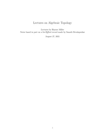
Circuit (tdm/fdm) vs. Packet switchingAverage Packet Service Time(slots)Average Service Time100TDM with 20sourcesIdeal l traffic load, packets per slotEytan ModianoSlide 221
M server systems: M/M/mbufferServerM serversλ packet per secondµ packet persecond, perserverServer Departure rate is proportional to the number of servers in useSimilar Markov chain:λδ1 λδ01µδEytan ModianoSlide 23λδλδ22µδm3µδλδλδmµδm 1mµδ
M/M/m queue Balance equations:!P(n " 1) nµP(n) n # m!P(n " 1) mµP(n) n m%' P(0)(m )n / n!n#mP(n) &,'( P(0)(mm n ) / m! n m Again, solve for P(0):"1 m "1 (m!) n(m! )m ')P(0) & # &% n 0 n!m!(1" !) )(P(0)(m!)mPQ # P(n) m!(1" !)n mn *mm !m n!NQ # nP(n m) # nP(0)() PQ ()m!1"!n 0n 0n *W Eytan ModianoSlide 24n *NQ, T W 1/ µ, N T / µ NQ !#1mµ
Applications of M/M/m Bank with m tellersNetwork with parallel transmission linesm lines, each of rate µλVSEytan ModianoSlide 25NodeBOne line of rate mµλ NodeANodeANodeBUseM/M/mformulaUseM/M/1formulaWhen the system is lightly loaded, PQ 0, and Single server is m times fasterWhen system is heavily loaded, queueing delay dominates and systems are roughly thesame
M/M/Infinity Unlimited servers customers experience no queueing delayThe number of customers in the system represents the number ofcustomers presently being servedλδ1 λδ0λδ1µδλδ22µδλδλδn3µδnµδn 1(n 1)µδP(0)(! / µ )n! P(n " 1) nµ P(n), #n 1, P(n) n!"1%P(0) '1 & n 1 (! / µ )n / n!) e" ! / µ(*P(n) (! / µ )n e" ! / µ / n! Poisson distribution!N Averagenumber in system ! / µ, T N / ! 1 / µ servicetimeEytan ModianoSlide 26
Blocking Probability A circuit switched network can be viewed as a Multi-server queueingsystem–– M/M/m/m system–– Calls are blocked when no servers available - “busy signal”For circuit switched network we are interested in the call blockingprobabilitym servers m circuitsLast m indicated that the system can hold no more than m usersErlang B formula––Gives the probability that a caller finds all circuits busyHolds for general call arrival distribution (although we prove Markov caseonly)PB Eytan ModianoSlide 27(! / µ) m / m!n(!/µ)/ n!"n 0m
M/M/m/m system: Erlang B formulaλδ1 λδ0λδ1µδλδλδ2m2µδ3µδmµδP(0)( ! / µ )n!P(n " 1) nµP(n), 1 # n # m, P(n) n!P(0) [%mn 0( ! / µ ) / n!n]"1(! / µ ) / m!PB P(Blocking ) P(m) m%n 0 (! / µ) n / n!mEytan ModianoSlide 28
Erlang B formula System load usually expressed in Erlangs–– A λ/µ (arrival rate)*(ave call duration) average loadFormula insensitive to λ and µ but only to their ratio(A) m / m!PB mn(A)/ n!!n 0Used for sizing transmission line––How many circuits does the satellite need to support?The number of circuits is a function of the blocking probability that we can tolerateSystems are designed for a given load predictions and blocking probabilities (typically small) Example–Arrival rate 4 calls per minute, average 3 minutes per call A 12–How many circuits do we need to provision?Depends on the blocking probability that we can tolerateEytan ModianoSlide 29CircuitsPB201571%8%30%
Multi-dimensional Markov Chains K classes of customers–Class j: arrival rate λj; service rate µj State of system: n (n1, n2, , nk); nj number of class j customers in the system If detailed balance equations hold for adjacent states, then a product form solutionexists, where:– P(n,.n2, , nk) P1(n1)*P2(n2)* *Pk(nk)Example: K independent M/M/1 systemsPi (ni ) ! ini (1 " ! i ), !i # i / µi Same holds for other independent birth-death chains–Eytan ModianoSlide 30E.g., M.M/m, M/M/Inf, M/M/m/m
Truncation Eliminate some of the states– E.g., for the K M/M/1 queues, eliminate all states where n1 n2 nk K1 (some constant)Resulting chain must remain irreducible–All states must communicateProduct form for stationary distribution of the truncated system E.g., K independent M/M/1 queues!1n1! 2n2 .! nKKP(n1, n2 ,.nk ) , G # !1n1! 2n2 .!Kn KGn"S E.g., K independent M/M/inf queues( !1n1 / n1!)(!2n2 / n2 !).(!Kn K / nk !)n1n2nKP(n1, n2 ,.nk ) , G # (!1 / n1!)( ! 2 / n2 !).( ! K / nk !)Gn"S––Eytan ModianoSlide 31G is a normalization constant that makes P(n) a distributionS is the set of states in the truncated system
Example Two session classes in a circuit switched system––M channels of equal capacityTwo session types:Type 1: arrival rate λ1 and service rate µ1Type 2: arrival rate λ2 and service rate µ2 System can support up to M sessions of either class–If µ1 µ2, treat system as an M/M/m/m queue with arrival rate λ1 λ2–––When µ1 ! µ2 need to know the number of calls in progress of each session typeTwo dimensional markov chain state (n1, n2)Want P(n1, n2): n1 n2 mCan be viewed as truncated M/M/Inf queues–Notice that the transition rates in the M/M/Inf queue are the same as those in a truncatedM/M/m/m queue( !1n1 / n1 !)( !2n2 / n2 !)P(n1, n2 ) ,G–Eytan ModianoSlide 32i m j m "iG #i 0#( ! / i!)(!j 0i1j2/ j!), n1 n2 mNotice that the double sum counts only states for which j i m
PASTA: Poisson Arrivals See Time Averages The state of an M/M/1 queue is the number of customers in the system More general queueing systems have a more general state that mayinclude how much service each customer has already received For Poisson arrivals, the arrivals in any future increment of time isindependent of those in past increments and for many systems of interest,independent of the present state S(t) (true for M/M/1, M/M/m, andM/G/1). For such systems, P{S(t) s A(t δ)-A(t) 1} P{S(t) s}– Eytan ModianoSlide 33(where A(t) # arrivals since t 0)In steady state, arrivals see steady state probabilities
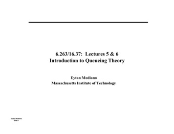
Occupancy distribution upon arrival Arrivals may not always see the steady-state averages Example:––Deterministic arrivals 1 per secondDeterministic service time of 3/4 secondsλ 1 packets/second T 3/4 seconds (no queueing)N λT Average occupancy 3/4 Eytan ModianoSlide 34However, notice that an arrival always finds the system empty!
Occupancy upon arrival for a M/M/1 queuean Lim t- inf (P (N(t) n an arrival occurred just after time t))Pn Lim t- inf (P(N(t) n))For M/M/1 systems an PnProof: Let A(t, t δ) be the event that and arrival occurred between t and t δan (t) Lim t- inf (P (N(t) n A(t, t δ) ) Lim t- inf (P (N(t) n, A(t, t δ) )/P(A(t, t δ) ) Lim t- inf P(A(t, t δ) N(t) n)P(N(t) n)/P(A(t, t δ) ) Since future arrivals are independent of the state of the system,P(A(t, t δ) N(t) n) P(A(t, t δ)) Hence, an (t) P(N(t) n) Pn(t) Taking limits as t- infinity, we obtain an Pn Result holds for M/G/1 systems as wellEytan ModianoSlide 35
Eytan Modiano Slide 10 Queueing Models Model for - Customers waiting in line - Assembly line - Packets in a network (transmission line) Want to know - Average number of customers in the system - Average delay experienced by a customer Quantities obtained in terms of - Arrival rate of customers (average number of customers per unit time) - Service rate (average number .