Transcription
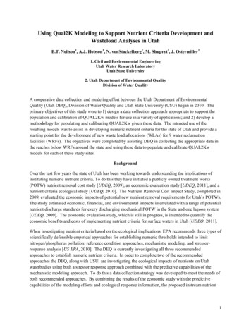
Using Qual2K Modeling to Support Nutrient Criteria Development andWasteload Analyses in UtahB.T. Neilson1, A.J. Hobson1, N. vonStackelberg2, M. Shupryt2, J. Ostermiller21. Civil and Environmental EngineeringUtah Water Research LaboratoryUtah State University2. Utah Department of Environmental QualityDivision of Water QualityA cooperative data collection and modeling effort between the Utah Department of EnvironmentalQuality (Utah DEQ), Division of Water Quality and Utah State University (USU) began in 2010. Theprimary objectives of this study were to 1) design a data collection approach appropriate to support thepopulation and calibration of QUAL2Kw models for use in a variety of applications; and 2) develop amethodology for populating and calibrating QUAL2Kw given these data. The intended use of theresulting models was to assist in developing numeric nutrient criteria for the state of Utah and provide astarting point for the development of new waste load allocations (WLAs) for 9 water reclamationfacilities (WRFs). The objectives were completed by assisting DEQ in collecting the appropriate data inthe reaches below WRFs around the state and using these data to populate and calibrate QUAL2Kwmodels for each of these study sites.BackgroundOver the last few years the state of Utah has been working towards understanding the implications ofinstituting numeric nutrient criteria. To do this they have initiated a publicly owned treatment works(POTW) nutrient removal cost study [UDEQ, 2009], an economic evaluation study [UDEQ, 2011], and anutrient criteria ecological study [UDEQ, 2010]. The Nutrient Removal Cost Impact Study, completed in2009, evaluated the economic impacts of potential new nutrient removal requirements for Utah’s POTWs.The study estimated economic, financial, and environmental impacts interrelated with a range of potentialnutrient discharge standards for every discharging mechanical POTW in the State and one lagoon system[UDEQ, 2009]. The economic evaluation study, which is still in progress, is intended to quantify theeconomic benefits and costs of implementing nutrient criteria for surface waters in Utah [UDEQ, 2011].When investigating nutrient criteria based on the ecological implications, EPA recommends three types ofscientifically defensible empirical approaches for establishing numeric thresholds intended to limitnitrogen/phosphorus pollution: reference condition approaches, mechanistic modeling, and stressorresponse analysis [US EPA, 2010]. The DEQ is currently investigating all three recommendedapproaches to establish numeric nutrient criteria. In order to complete two of the recommendedapproaches the DEQ, along with USU, are investigating the ecological impacts of nutrients on Utahwaterbodies using both a stressor response approach combined with the predictive capabilities of themechanistic modeling approach. To do this a data collection strategy was developed to meet the needs ofboth recommended approaches. By combining the results of the economic study with the predictivecapabilities of the modeling efforts and ecological response information, the proposed instream nutrient1
criteria can be linked to the expected economic costs of the treatment upgrades as well as forecasting thepotential impact of nutrient loading on the ecological health of the downstream waterbodies.This report covers the general approaches taken in the mechanistic modeling portion of the NutrientCriteria study for data collection, model population, and calibration/validation. However, it is importantto note that the data collection approaches and models are intended to have multiple applications andtherefore, have been made very generic in order to support: 1) development of statewide numeric nutrientcriteria; 2) development of site-specific criteria for rivers and streams where the statewide nutrient criteriado not appear valid; 3) wasteload analyses to determine water quality based effluent limits (WQBEL), and4) determination of TMDL endpoints. Details regarding the associated ecological measures and referencecondition information can be found at UAL2Kw ModelUtah DEQ uses low flow conditions to determine WQBELs for point sources under the Utah PollutionDischarge Elimination System (UPDES) program (UDEQ, 2012) due in part to these corresponding withlimiting conditions. This led to selecting a model that would be appropriate for these conditions.QUAL2K [Chapra et al., 2004] is a USEPA approved model that has been commonly used in WLAs andtotal maximum daily loads (TMDLs) (e.g., [Bischoff et al., 2010; Kardouni and Cristea, 2006]), and evendevelopment of nutrient criteria [Flynn and Suplee, 2011]. This quasi-dynamic, one dimensional instreamwater quality model includes the dominant processes of concern within Utah waters, predicts the requiredwater quality variables, and is feasible to populate and calibrate given the limited data available in mostwaterbodies of the state. In order to understand the associated daily minimum and maximum instreamconcentrations, the model provides a 24 hour diel response in water quality given an appropriate orrepresentative 24 hour weather pattern. QUAL2Kw [Pelletier and Chapra, 2008], a sister model toQUAL2K developed within the state of Washington, built in additional functionality (e.g., automaticcalibration algorithms) into QUAL2K based on their identified needs. With the anticipation of havingsome similar needs as Washington and the possibility of identifying additional needs, Utah DEQ electedto use QUAL2Kw in their instream modeling applications.Details regarding the version of QUAL2Kw used in this application (version 5.1) are provided within theuser's manual [Pelletier and Chapra, 2008] and a number of publications [Cho and Ha, 2010; Kannel etal., 2007; Pelletier et al., 2006]. In short, the state variables (Table 1) include the macro nutrients (C, N,and P) of interest and the critical nutrient species (e.g., inorganic P, nitrate, and ammonia) in surfacewaters.Using the same notation as that of Table 1, the QUAL2Kw composite or calculated variables are(Pelletier and Chapra, 2008):Total Organic Carbon (mgC/L):TOC cs c froc rca a p rcd mo(1)2
Table 1. QUAL2Kw State Variables (taken directly from [Pelletier and Chapra, 2008]).VariableConductivityInorganic suspended solidsDissolved oxygenSlow-reacting CBODFast-reacting CBODOrganic nitrogenAmmonia nitrogenNitrate nitrogenOrganic phosphorusInorganic phosphorusPhytoplanktonDetritusPathogenGeneric constituentAlkalinityTotal inorganic carbonBottom algae (ab in the surface water layer),biofilm of attached heterotrophic bacteria(ah in the hyporheic sediment zone for the Level 2 option)Bottom algae nitrogenBottom algae phosphorus* mg/L g/m3SymbolUnits* mhoss1, s2mgD/Lmi,1, mi,2mgO2/Lo1, o2mg O2/Lcs,1, cs,2mg O2/Lcf,1, cf,2 gN/Lno,1, no,2 gN/Lna,1, na,2 gN/Lnn,1, nn,2 gP/Lpo,1, po,2 gP/Lpi,1, pi,2 gA/Lap,1, ap,2mgD/Lmo,1, mo,2cfu/100 mLx1, x2gen1, gen2 user definedAlk1, Alk2 mgCaCO3/Lmole/LcT,1, cT,2gD/m2ab,ahINbIPbmgN/m2mgP/m2Total Nitrogen ( gN/L):TN no n a n n rna a p(2)Total Phosphorus ( gP/L):TP po pi rpa a p(3)Total Kjeldahl Nitrogen ( gN/L):TKN no na rna a p(4)Total Suspended Solids (mgD/L):TSS rda a p mo mi(5)Ultimate Carbonaceous BOD (mgO2/L):CBODu c s c f roc rca a p roc rcd mo(6)3
Additionally, the model provides the ability to predict the associated biological effects of various nutrientconcentrations since photosynthesis, respiration, and death of phytoplankton and bottom algae areincluded within the model. As the version of QUAL2Kw applied within this study is quasi-dynamic, itprovides the ability to deal with steady flow, but does allow for non-uniform flow. This means that whilethe flow conditions cannot change over time, they can vary longitudinally downstream due to point ordistributed inflows or abstractions.Given the capabilities of this version of QUAL2Kw, there are environmental conditions that are suitedfor this type of modeling approach. The time period over which this model should be applied require that1) stream conditions are completely mixed since the model assumes all model elements are completelymixed, 2) boundary condition concentrations can be approximated by consistent 24 hourly values; 3)distributed flows are constant, 4) point inflows follow a consistent diel pattern or are constant, and 5)weather conditions over the simulation period have a consistent diel pattern.Study Site LocationsNine sites were selected for the nutrient criteria ecological study and represent the different types ofreceiving waterbodies around the state of Utah (Figure 1). Using these sites as a representative sample ofthe state’s waterbodies, the QUAL2Kw, ecological stressor-response, and reference condition findingswill be used to extrapolate information regarding possible ranges of nutrient criteria for the remainingstate waters [UDEQ, 2010]. The selected sites (Table 2) are located within different order streams withvaried background water quality, surrounding land uses, and amounts of wastewater effluent that havebeen treated to different levels. The sections studied were those influenced by WRF effluents since theseareas generally have enhanced nutrient loads. More detail regarding each site (e.g., location, study reachlength, etc.) are provided in a separate report in preparation by the Division of Water Quality thatevaluates structural and functional responses to nutrients. Detailed information about unique samplingrequirements associated with each site and the specific information regarding model population,calibration, and validation are provided within the QUAL2K modeling files and site specific modeldocumentation provided to Utah DEQ as project deliverables (see Appendix B for an example).Figure 1. Study site locations within the state of Utah.4
Table 2. Study site locations, water reclamation facilities, and dates sampled within the state of Utah.WaterbodyFacilityDates SampledBox Elder CreekBrigham City WRFAug. 9 - 11, 2010San Pitch RiverFairview City WRFAug. 2 - 5, 2010Oct. 11 - 13, 2010July 28-30, 2010San Pitch RiverMoroni City WRFWeber RiverOakley City WRFAug 23-26, 2010Price RiverPrice River Water Improvement DistrictAug. 30 - Sep 1, 2010Dry CreekSpanish Fork City WRFJuly 23 - 26, 2010Silver CreekSnyderville Basin-Silver Creek Water Reclamation FacilityMalad RiverTremonton City WRFJuly 20 - 22, 2010Sep. 30 - Oct 4, 2010Aug 22-30, 2011Aug. 13 - 16, 2010Little Bear RiverWellsville LagoonsSept 10-13, 2010Project ResultsSince the key objectives in this project were to develop the appropriate data collection methodologies tosupport QUAL2Kw model population and calibration, this report provides general information regardingthe field data requirements, approaches to model population using these data, strategies used in modelcalibration, and the steps required for model validation (if these data sets exist).Supporting field dataData must be collected at 3 general locations for instream modeling. The beginning of the study reach(also called the headwater or upstream boundary condition), inflows/outflows (point sources or tributaryinflows and diversions/abstractions), and at least one location downstream for model calibration. Thedata types required at these locations will vary and are discussed below. For the 2010 data collectionefforts, data collection at each location spanned a 2 day period during low flow conditions.Figure 2 shows a generalized schematic used within the 2010 data collection efforts. Data for themodeling efforts were gathered at Station B (headwater/upstream boundary condition), Station C(wastewater treatment plant effluent before it enters the stream), Station D (at a location where the streamand point source effluent was completely mixed), and Station E (the calibration location downstream atthe end of the study reach). Information gathered at Station A was only used in the ecological portion ofthe study. If a tributary entered the modeling reach, data were also collected at T1. Similarly, if adiversion was present, the quantity of water leaving the system was determined.5
POTW1.2.3.4.5.6.Water Quality SondeTEMPERATURE*SPEC. CONDUCTANCE*DISSOLVED OXYGEN*CHLOROPHYLL APHTURBIDITYA2B2C1.2.3.4.5.6.Chemistry Grab SamplesCARB. BOD 5CHLOROPHYLL‐APHSPEC. CONDUCTANCETOTAL SUSPENDED SOLIDSTOTAL ALKALINITY1.2.3.4.5.Nutrient Grab SamplesAMMONIA as NNITRITE NITRATE as NTOTAL NITROGENPHOSPHATE as PTOTAL PHOSPHORUSPOTW2Reaeration LengthD22T1D1E22Total Sonde*Partial Sonde2 Day Grab SampleFlow MeasurementFigure 2. Generalized data collection locations within the 2010 sampling efforts. Requiredlocations of flow measurements and the multi-parameter water quality sondes are also shown.Since 2010 modeling efforts used Station B as the headwater location, the information forchlorophyll-a and pH is taken from Station A.For the 2010 data collection, the location of the completely mixed conditions downstream of the WRFwas determined by measuring specific conductance or temperature across the channel to determine whereuniform conditions existed. In some cases where the differences in temperature and/or specificconductance were too small, rhodamine WT was used as a visual indicator. To support and integrate theseefforts with the ecological study needs the distance between Station D and E was estimated using methodsdescribed in Grace and Imberger [2006] which designate the optimum distance between stations forcalculating open water metabolism using the single station method (Eqn. 7).X 0.693 vv 0.33 k a 0.0137 D 0.85 (7)Where X optimum station distance (km), v velocity (cm s ¹), D depth (cm), and ka reaerationcoefficient for oxygen (d-1). As discussed later, we found this method to result in distances that were ingeneral too short to meet the diverse needs of this study and often times did not include the compliancepoint for WLAs.The information necessary at each of these stations is dependent on whether it is the headwater location, aload, or a diversion. Water quality models require an understanding of both the water balance and themass balances for each constituent modeled. Flow measurements may be required at all stations in orderto establish a water balance. Water quality information is not, however, required for diversions or6
abstractions since the mass loss will be a function of the instream concentrations predicted by the modeland the volume of water taken out that is specified by the user.The specific water quality constituents measured at each station and the frequency they were collected aredetailed within Table 3. There are a number of constituents that were measured using multi-parametersondes (e.g., temperature, dissolved oxygen, conductivity) at five minute increments over each of the twoday sampling period. Grab samples of most constituents requiring laboratory analyses were gatheredeach day and usually in the mid-morning. Benthic algae sampling was only conducted once at some pointin time close to the study periods. A number of constituents within this list, indicated by a * in the table,were not sampled directly and had to be estimated. The appropriate values for modeling were estimatedusing the relationships between measured constituents and model variables as described below.Additional data types that could be collected that would be useful in the modeling include a measure ofsediment oxygen demand, total organic carbon, and volatile suspended solids. None of these measureswere completed in the 2010 data sets.Data to characterize each site is additionally necessary to support model population or calibration. Table4 provides a list of the data types requiring collection, some procedural information, locations where thesedata are required within or near the site, and the utility of the data in the context of the modeling effort. Anumber of these data types are collected within routine Utah’s Comprehensive Assessment of StreamEcosystems (UCASE) surveys based on protocols adapted from the USEPA [2007]. It is important tonote that all locations where data are collected must have GPS coordinates established for documentationpurposes.Model PopulationOnce the data have been collected, they must be translated from observations to model inputs. The modelstate variables (Table 1) can be related to measurements as follows [taken directly from Pelletier andChapra, 2008]:Conductivity s COND(8)ISS mi TSS – VSS or TSS – rdc (TOC – DOC)(9)Dissolved Oxygen o DO(10)Organic Nitrogen no TKN – NH4 – rna CHLAor(11)no TN – NO2 – NO3 – NH4 – rna CHLAAmmonia Nitrogen na NH4(12)Nitrate Nitrogen nn NO2 NO3(13)Organic Phosphorus po TP – SRP – rpa CHLA(14)Inorganic Phosphorus pi SRP(15)Phytoplankton ap CHLA(16)7
Table 3. Water quality constituents sampled and the frequency of sampling for QUAL2Kwmodeling.Multi-Parameter Sonde DataAbbreviation/QUAL2Kw UnitsFrequencyWater TemperatureTemp ( C)5 min samplesSpecific ConductanceCOND (mhos)5 min samplesDissolved OxygenDO (mgO2/L)5 min samplespHpH5 min samplesChlorophyll aCHLA ( gA/L)5 min samplesTurbidity5 min samplesLaboratory Analysis5-Day Soluble Carbonaceous BOD, sCBOD51 each dayTotal NitrogenTN (gN/L)1 each dayAmmonia NitrogenNH4 (gN/L)1 each dayNitrate Nitrite NitrogenNO3 (gN/L)1 each dayTotal PhosphorusTP (gP/L)1 each daySoluble Reactive PhosphorusSRP (gP/L)1 each dayVolatile Suspended Solids*VSS (mgD/L)1 each dayTotal Suspended SolidsTSS (mgD/L)1 each dayAlkalinityALK (mgCaCO3/L)1 each dayChlorophyll aCHLA (gA/L)1 each dayDissolved Organic Carbon, DOCDOC (mgC/L)1 each dayDissolved Organic Phosphorus, DOP*1 each dayDissolved Organic Nitrogen, DON*1 each dayBenthic Chl-a1 per sampling time periodBenthic AFDM1 per sampling time periodBenthic TP1 per sampling time periodBenthic TN1 per sampling time periodBenthic TOC1 per sampling time period#SOD#TOC1 per sampling time periodTOC (mgC/L)1 each day* not gathered or required estimation for QUAL2Kw# data that would be useful in model population/calibration but were not directly measured in these efforts8
Table 4. Site characterization data types.Data TypeAverage CrossSectionalVelocity*ProcedureSee methods provided withinData Collection and/or UCASESOP. Information from HECRAS modeling applications canalso be extracted to supplementdata collected.LocationsStation D, E, and above and belowany inflow or outflow. Additionallocations along study reach would bebeneficial.Station D, E, and above and belowany inflow or outflow. Additionallocations along study reach would bebeneficial.AverageChannel BottomWidthSee methods provided withinData Collection and/or UCASESOP.Bottom width estimates werecalculated using side slope,average depth, and top widthvalues in the formula: TopWidth – Depth x1/tan(radians( SSLEW)) –Depth x 1/tan(radians( SSREW)), where width anddepth are in meters and sideslope is in radians in the formof Run/Rise.Channel BottomSlopeSee methods provided withinUCASE SOP.Channel SideSlopeSee methods provided withinUCASE SOP.Station D, E, and above and belowany inflow or outflow. Additionallocations along study reach would bebeneficial.Should estimate bottom slope frombeginning to end of study reach at10% increments of total reach lengthand/or when changes in bottom slopeare observed.Station D, E, and above and belowany inflow or outflow. Additionallocations along study reach would bebeneficial.Weather dataOnsite weather station ornearest Mesowest Station.Near study site would be mostappropriate and 15-30 minute data arepreferred.Tracer StudyInject tracer at Station B or Cand measure response atStation E. Can also use HECRAS model if available.Substrate type*See methods provided withinData Collection and/or UCASESOP.Measure tracer response at Station E,but additional locations along thestudy reach would be beneficial tocapture heterogeneity.Information should be gathered atcross sections in subreaches thatrepresent the variability in substratetypes.Shading*See methods provided withinData Collection and/or UCASESOP.Information should be gathered atlocations that represent the variabilityin shading.Average CrossSectional Depth*ReasoningProvides observations of velocity indifferent reaches to compare with thepredicted velocities. This can be usedwith the depth and tracer information toensure appropriate representation of thehydraulics and reasonable travel times.Provides observations of depths indifferent reaches to compare with thepredicted depths. This can be used withthe velocity and tracer information toensure appropriate representation of thehydraulics and reasonable travel times.Model input.Model input.Model input and can be used tocalculate bottom width from measuredtop widths.Wind speed, air temperature, shortwavesolar radiation, humidity/dewpointtemperature are all used within themodel as forcing information.Precipitation data shows whether therewas significant rainfall in the area thatwould influence instream flows.Provides information regarding averagetravel time through system and can beused in calibration of hydraulicparameters (e.g., Manning’s roughnesscoefficient).Provides a method to approximate theMannings roughness coefficient anddetermine fraction of bottom substrateappropriate for bottom algae.Model input. If riparian or topographicshading drastically influences instreamtemperatures, estimates of the shading% for each hour of a day will benecessary to scale the incomingshortwave solar radiation.9
Detritus mo VSS – rda CHLA or rdc (TOC – DOC) – rda CHLA(17)pH PH(18)Alkalinity Alk ALK(19)While a number of these relationships are straightforward, it is important to realize that the typicalOrganic N and Organic P measurement cannot be directly compared to the Organic N and Organic PQUAL2Kw predictions. As shown in equations 11 and 14 above, the QUAL2Kw versions of organic Nand P only represent the dissolved and detritus portion of each organic nutrient pool since the portionassociated with the live algae are subtracted out. It is also important to note that detritus (Eqn 17) onlycontributes to the carbon budget and does not influence other nutrient pools.Given the data available from the 2010 sampling, we needed additional methods based on someassumptions or established equations to calculate the variables necessary for model population andcalibration. These included the need to convert sCBOD5 measurements to the sCBOD ultimate valuesrequired within QUAL2Kw (Eqn 20).sCBOD ultimate cf or cs sCBOD5/(1-exp(-kd (5days))(20)Further, since we did not have direct measures of VSS or ISS in the 2010 data sets, we had to come upwith methods and a logic tree to estimate these values for model population (Figure 3).Inorganic Suspended SolidsISSIf VSS TSS, ISS 15 % TSSTotal Suspended SolidsTSS(Measured)Else, ISS TSS ‐ VSSChlorophyll a (VSSlive)Organic Suspended Solids(Measured)VSS(live dead)If VSS TSS, VSS TSS – ISSElse VSS (Org. N, P)(Total –Diss.) X r D:(N,P)Detritus (VSS dead)If VSS Cha x r D:A,Detritus VSS – Cha X rD:AElse, Detritus 0Figure 3. Logic used in estimating VSS and ISS from TSS, followed by logic for estimating detritus fromVSS.To populate the model, information regarding the reach, initial conditions, headwater conditions, weatherdata, point sources and distributed sources must be provided (Table 5). More specifically, observationsfrom the headwater location and any point flow (inflow or abstraction) or distributed flows must beentered into the model framework. Any flow information provided for these locations must be arepresentative value for the entire modeling period. The necessary sampling frequency of specific waterquality data is dependent upon whether it is a point source or headwater (Table 6). The other forcing data10
Table 5. General information required for QUAL2Kw model population.QUAL2Kw SheetReachInformation RequiredReach segmentationHydraulic characteristics% suitable substrateBottom algae % coverSODThermal propertiesInitial ConditionsConstituent concentrations (See Table 6)Headwater DataAverage flowConstituent concentrations (See Table 6)Weather Data(hourly average values)Air temperatureDewpoint temperatureSolar radiationShadingCloud coverWind speedPoint SourcesAverage flowConstituent concentrations (See Table 6)Distributed SourcesAverage flowConstituent concentrations (See Table 6)RatesPrimarily set in calibration.See Model Calibration section below.Table 6. Model input constituent concentrations requirements and the associated observed dataused in population of QUAL2Kw.Point SourceHeadwaterDistributed InflowAverageModel ParameterData CollectedMean Range/2 or 2 Day MeanHourly Averageor 2 Day MeanAlkalinityTotal AlkalinityXXXsCBODultimatesCBOD5XXXSpecific ConductivitySpecific ConductivityXXXDetritus (POM)(Org - Diss. N, P) X r(POM/N, P)XXXDissolved OxygenDissolved OxygenXXXInorganic Phosphorus (SRP)Inorganic Phosphorus (SRP)XXXInorganic SolidsTSS - itrogenXXXOrganic NitrogenTN - (NH4) - (NO3 NO2)XXXOrganic PhosphorusTP - Inorg PXXXpHpHXXXPhytoplanktonChlorophyll aXXXWater TemperatureWater TemperatureXXX11
required by the model is meteorological information which includes hourly average air temperatures,wind speeds, and dewpoint temperatures from a nearby, representative weather station. Shortwave solarradiation can be estimated automatically within the modeling framework, however, if using theseestimates, hourly cloud cover values would be required. In the 2010 modeling efforts, we instead usedactual shortwave radiation observations from a local source.When populating the models, censored data, or concentrations that are below the analytical detectionlimits (i.e., non-detects) commonly occur. Within the 2010 modeling, non-detects were assigned aconcentration of half of the detection limit. More accurate statistical analysis of limited amounts ofcensored data should be investigated. The detection limits associated with key parameters are detailedwithin Table 7.Table 7. Detection limits for constituents based on the procedures applied within specific laboratories.ConstituentTN, TPTDN, TDPNO3 NO2 -NNH4 -NPO4 -PsCBOD5Chlorophyll aSpecific ConductanceTotal Suspended SolidsTotal Dissolved Solids (180 C)TurbidityLaboratoryBaker Lab – USUBaker Lab – USUBaker Lab – USUBaker Lab – USUBaker Lab – USUUtah DEQ Laboratory/AWALUtah DEQ LaboratoryUtah DEQ LaboratoryUtah DEQ LaboratoryUtah DEQ LaboratoryUtah DEQ LaboratoryAnalytical DetectionLimit (mg/L)0.00570.00250.00060.003950.00083/50.00072 (uS/cm)4100.1 (NTU)To assist in ensuring model population consistency given the relatively consistent data collectionstrategies implemented in 2010, we developed two supporting sheets within the QUAL2Kw filesdelivered to DEQ. A "Data Input" and "Addt Info" sheet provides a number of tables that can bepopulated with observations, and this information automatically populates the QUAL2Kw sheets.Further, these sheets facilitate some of the additional calculations that were completed and suggested infuture applications (described further below). Information regarding these features is included withinAppendix A.Most information within the Rates Sheet was not changed at all or was adjusted in model calibration(described further below). However, specific values of some parameters were established within the 2010modeling efforts that may be appropriate for other Utah model applications. First, we measured CBODdecomposition rates (kd) by taking 6 samples from the Silver Creek WRF effluent. These samples wereanalyzed in triplicate resulting in 18 total measurements of 30 day CBOD using methods detailed inEnvironmental Protection Division [1989]. The resulting data were analyzed using a Nonlinear LeastSquares Method and the Thomas Method (Table 8). Given that Chapra [1997] reports values ranging0.05-0.1 d-1 at 20 C for waste streams treated using activated sludge, we assumed the average value of0.103 d-1 was an appropriate value for all the 2010 study sites and this value was not varied in calibration.Further, this value was used to convert any measured concentrations of sCBOD5 to the sCBOD ultimatevalues required by the model (Table 6). We do, however, suggest that a Utah specific number be12
established for the dominant wastewater treatment types of activated sludge and membrane mechanicaltreatment as well as for lagoon systems.Table 8. CBOD decomposition rate statistics based on samples from Silver Creek WRF effluent.MinMaxMeanStDev95% CINLS Methodkd, 1/d0.0950.1250.1030.0110.013Thomas Methodkd, 1/d0.0760.1240.0960.0120.013The thermal properties of the Silver Creek substrate were also measured since these dictate the rate ofheat exchange between the water column and the sediments. While there are a number of values reportedwithin the QUAL2K and QUAL2Kw manual, it can be important to have site specific thermal properties.The thermal property values based on measurements from Silver Creek with a sandy-gravel substratewere a thermal diffusivity of 0.72 mm2 s-1 and a thermal conductivity of 2.25 W m-1 k-1.Model CalibrationCalibration within this effort consisted of a number of manual calibration steps followed byautocalibration using the genetic algorithm within QUAL2Kw. The data used in calibration includedhydraulics data (longitudinal depths, velocities, and travel time) and water quality data (Table 3)including the mean, minimum, and maximum values at each calibration location (only station E for the2010 effort). For those data types where only 2 samples were taken, the minimum and maximum valueswere not always representative of the daily variability and only provided an understanding of the range atthese sampling times.Manual Calibration StepsA number of manual calibration steps and or checks were identified to ensure that the model wasrepresenting the system well based
By combining the results of the economic study with the predictive capabilities of the modeling efforts and ecological response information, the proposed instream nutrient . As the version of QUAL2Kw applied within this study is quasi-dynamic, it provides the ability to deal with steady flow, but does allow for non-uniform flow. This means .