Transcription
Open Source Tools forOptimization in PythonTed RalphsSciPy 2015IIT Bombay, 16 Decmber 2015T.K. Ralphs (Lehigh University)COIN-ORDecember 16, 2015
Outline1Introduction2PuLP3Pyomo4Solver Studio5Advanced ModelingSensitivity AnalysisTradeoff Analysis (Multiobjective Optimization)Nonlinear ModelingInteger ProgrammingStochastic ProgrammingT.K. Ralphs (Lehigh University)COIN-ORDecember 16, 2015
Outline1Introduction2PuLP3Pyomo4Solver Studio5Advanced ModelingSensitivity AnalysisTradeoff Analysis (Multiobjective Optimization)Nonlinear ModelingInteger ProgrammingStochastic ProgrammingT.K. Ralphs (Lehigh University)COIN-ORDecember 16, 2015
Algebraic Modeling LanguagesGenerally speaking, we follow a four-step process in modeling.Develop an abstract model.Populate the model with data.Solve the model.Analyze the results.These four steps generally involve different pieces of software working inconcert.For mathematical programs, the modeling is often done with an algebraicmodeling system.Data can be obtained from a wide range of sources, including spreadsheets.Solution of the model is usually relegated to specialized software, depending onthe type of model.T.K. Ralphs (Lehigh University)COIN-ORDecember 16, 2015
Open Source Solvers: COIN-ORThe COIN-OR FoundationA non-profit foundation promoting the development and use ofinteroperable, open-source software for operations research.A consortium of researchers in both industry and academia dedicated toimproving the state of computational research in OR.A venue for developing and maintaining standards.A forum for discussion and interaction between practitioners andresearchers.The COIN-OR RepositoryA collection of interoperable software tools for building optimizationcodes, as well as a few stand alone packages.A venue for peer review of OR software tools.A development platform for open source projects, including a wide rangeof project management tools.T.K. Ralphs (Lehigh University)COIN-ORDecember 16, 2015
The COIN-OR Optimization SuiteCOIN-OR distributes a free and open source suite of software that can handle allthe classes of problems we’ll discuss.Clp (LP)Cbc (MILP)Ipopt (NLP)SYMPHONY (MILP, BMILP)DIP (MILP)Bonmin (Convex MINLP)Couenne (Non-convex MINLP)Optimization Services (Interface)COIN also develops standards and interfaces that allow software components tointeroperate.Check out the Web site for the project at http://www.coin-or.orgT.K. Ralphs (Lehigh University)COIN-ORDecember 16, 2015
Installing the COIN-OR Optimization SuiteSource builds out of the box on Windows, Linux, OSX using the Gnu autotools.Packages are available to install on many Linux distros, but there are somelicensing issues.Homebrew recipes are available for many projects on OSX (we are working onthis).For Windows, there is a GUI installer zationSuite/For many more details, see Lecture 1 of this tutorial:http://coral.ie.lehigh.edu/ ted/teaching/coin-orT.K. Ralphs (Lehigh University)COIN-ORDecember 16, 2015
Modeling SoftwareMost existing modeling software can be used with COIN solvers.Commercial SystemsGAMSMPLAMPLAIMMSPython-based Open Source Modeling Languages and InterfacesPyomoPuLP/DippyCyLP (provides API-level interface)yaposibT.K. Ralphs (Lehigh University)COIN-ORDecember 16, 2015
Modeling Software (cont’d)Other Front Ends (mostly open source)FLOPC (algebraic modeling in C )CMPLMathProg.jl (modeling language built in Julia)GMPL (open-source AMPL clone)ZMPL (stand-alone parser)SolverStudio (spreadsheet plug-in: www.OpenSolver.org)Open Office spreadsheetR (RSymphony Plug-in)Matlab (OPTI)MathematicaT.K. Ralphs (Lehigh University)COIN-ORDecember 16, 2015
How They InterfaceAlthough not required, it’s useful to know something about how modelinglanguages interface with solvers.In many cases, modeling languages interface with solvers by writing out anintermediate file that the solver then reads in.It is also possible to generate these intermediate files directly from acustom-developed code.Common file formatsMPS format: The original standard developed by IBM in the days of Fortran, noteasily human-readable and only supports (integer) linear modeling.LP format: Developed by CPLEX as a human-readable alternative to MPS.nl format: AMPL’s intermediate format that also supports non-linear modeling.OSIL: an open, XML-based format used by the Optimization Services framework ofCOIN-OR.Several projects use Python C Extensions to get the data into the solver throughmemory.T.K. Ralphs (Lehigh University)COIN-ORDecember 16, 2015
Where to Get the ExamplesThe remainder of the talk will review a wide range of examples.These and many other examples of modeling with Python-based modelinglanguages can be found at the below sT.K. Ralphs (Lehigh University)COIN-ORDecember 16, 2015
Outline1Introduction2PuLP3Pyomo4Solver Studio5Advanced ModelingSensitivity AnalysisTradeoff Analysis (Multiobjective Optimization)Nonlinear ModelingInteger ProgrammingStochastic ProgrammingT.K. Ralphs (Lehigh University)COIN-ORDecember 16, 2015
PuLP: Algebraic Modeling in PythonPuLP is a modeling language in COIN-OR that provides data types for Pythonthat support algebraic modeling.PuLP only supports development of linear models.Main classesLpProblemLpVariableVariables can be declared individually or as “dictionaries” (variables indexed onanother set).We do not need an explicit notion of a parameter or set here because Pythonprovides data structures we can use.In PuLP, models are technically “concrete,” since the model is always createdwith knowledge of the data.However, it is still possible to maintain a separation between model and data.T.K. Ralphs (Lehigh University)COIN-ORDecember 16, 2015
Simple PuLP Model (bonds simple-PuLP.py)from pulp import LpProblem, LpVariable, lpSum, LpMaximize, valueprob LpProblem("Dedication Model", LpMaximize)X1 LpVariable("X1", 0, None)X2 LpVariable("X2", 0, None)probprobprobprob 4*X1X1 2*X13*X1 3*X2X2 100 X2 150 4*X2 360prob.solve()print ’Optimal total cost is: ’, value(prob.objective)print "X1 :", X1.varValueprint "X2 :", X2.varValueT.K. Ralphs (Lehigh University)COIN-ORDecember 16, 2015
PuLP Model: Bond Portfolio Example (bonds-PuLP.py)from pulp import LpProblem, LpVariable, lpSum, LpMaximize, valuefrom bonds import bonds, max rating, max maturity, max cashprob LpProblem("Bond Selection Model", LpMaximize)buy LpVariable.dicts(’bonds’, bonds.keys(), 0, None)prob lpSum(bonds[b][’yield’] * buy[b] for b in bonds)prob lpSum(buy[b] for b in bonds) max cash, "cash"prob (lpSum(bonds[b][’rating’] * buy[b] for b in bonds) max cash*max rating, "ratings")prob (lpSum(bonds[b][’maturity’] * buy[b] for b in bonds) max cash*max maturity, "maturities")T.K. Ralphs (Lehigh University)COIN-ORDecember 16, 2015
PuLP Data: Bond Portfolio Example (bonds data.py)bonds {’A’ : {’yield’: 4,’rating’: 2,’maturity’ : 3,},’B’ : {’yield’: 3,’rating’: 1,’maturity’ : 4,},}max cash 100max rating 1.5max maturity 3.6T.K. Ralphs (Lehigh University)COIN-ORDecember 16, 2015
Notes About the ModelWe can use Python’s native import mechanism to get the data.Note, however, that the data is read and stored before the model.This means that we don’t need to declare sets and parameters.ConstraintsNaming of constraints is optional and only necessary for certain kinds ofpost-solution analysis.Constraints are added to the model using an intuitive syntax.Objectives are nothing more than expressions without a right hand side.IndexingIndexing in Python is done using the native dictionary data structure.Note the extensive use of comprehensions, which have a syntax very similar toquantifiers in a mathematical model.T.K. Ralphs (Lehigh University)COIN-ORDecember 16, 2015
Notes About the Data ImportWe are storing the data about the bonds in a “dictionary of dictionaries.”With this data structure, we don’t need to separately construct the list of bonds.We can access the list of bonds as bonds.keys().Note, however, that we still end up hard-coding the list of features and we mustrepeat this list of features for every bond.We can avoid this using some advanced Python programming techniques, buthow to do this with SolverStudio later.T.K. Ralphs (Lehigh University)COIN-ORDecember 16, 2015
Bond Portfolio Example: Solution in PuLPprob.solve()epsilon .001print ’Optimal purchases:’for i in bonds:if buy[i].varValue epsilon:print ’Bond’, i, ":", buy[i].varValueT.K. Ralphs (Lehigh University)COIN-ORDecember 16, 2015
Example: Short Term FinancingA company needs to make provisions for the following cash flows over the comingfive months: 150K, 100K, 200K, 200K, 300K.The following options for obtaining/using funds are available,The company can borrow up to 100K at 1% interest per month,The company can issue a 2-month zero-coupon bond yielding 2% interest over thetwo months,Excess funds can be invested at 0.3% monthly interest.How should the company finance these cash flows if no payment obligations areto remain at the end of the period?T.K. Ralphs (Lehigh University)COIN-ORDecember 16, 2015
Example (cont.)All investments are risk-free, so there is no stochasticity.What are the decision variables?xi , the amount drawn from the line of credit in month i,yi , the number of bonds issued in month i,zi , the amount invested in month i,What is the goal?To maximize the cash on hand at the end of the horizon.T.K. Ralphs (Lehigh University)COIN-ORDecember 16, 2015
Example (cont.)The problem can then be modeled as the following linear program:max(x,y,z,v) R12f (x, y, z, v) vs.t. x1 y1 z1 150x2 1.01x1 y2 z2 1.003z1 100x3 1.01x2 y3 1.02y1 z3 1.003z2 200x4 1.01x3 1.02y2 z4 1.003z3 200 1.01x4 1.02y3 v 1.003z4 300100 xi 0 (i 1, . . . , 4)xi 0(i 1, . . . , 4)yi 0(i 1, . . . , 3)zi 0(i 1, . . . , 4)v 0.T.K. Ralphs (Lehigh University)COIN-ORDecember 16, 2015
PuLP Model for Short Term Financing(short term financing-PuLP.py)from short term financing data import cash, c rate, b yieldfrom short term financing data import b maturity, i rateT len(cash)credit LpVariable.dicts("credit", range(-1, T), 0, None)bonds LpVariable.dicts("bonds", range(-b maturity, T), 0, None)invest LpVariable.dicts("invest", range(-1, T), 0, None)prob invest[T-1]for t in range(0, T):prob (credit[t] - (1 c rate)* credit[t-1] bonds[t] - (1 b yield) * bonds[t-int(b maturity)] invest[t] (1 i rate) * invest[t-1] cash[t])prob credit[-1] 0prob credit[T-1] 0prob invest[-1] 0for t in range(-int(b maturity), 0): prob bonds[t] 0for t in range(T-int(b maturity), T): prob bonds[t] 0T.K. Ralphs (Lehigh University)COIN-ORDecember 16, 2015
More Complexity: Facility Location ProblemWe have n locations and m customers to be served from those locations.There is a fixed cost cj and a capacity Wj associated with facility j.There is a cost dij and demand wij for serving customer i from facility j.We have two sets of binary variables.yj is 1 if facility j is opened, 0 otherwise.xij is 1 if customer i is served by facility j, 0 otherwise.Capacitated Facility Location Problemmins.t.nXj 1nXj 1mXcj yj m XnXdij xiji 1 j 1xij 1 iwij xij Wj ji 1xij yjxij , yj {0, 1}T.K. Ralphs (Lehigh University)COIN-OR i, j i, jDecember 16, 2015
PuLP Model: Facility Location Examplefrom productsimport REQUIREMENT, PRODUCTSfrom facilities import FIXED CHARGE, LOCATIONS, CAPACITYprob LpProblem("Facility Location")ASSIGNMENTS [(i, j) for i in LOCATIONS for j in PRODUCTS]assign vars LpVariable.dicts("x", ASSIGNMENTS, 0, 1, LpBinary)use vars LpVariable.dicts("y", LOCATIONS, 0, 1, LpBinary)prob lpSum(use vars[i] * FIXED COST[i] for i in LOCATIONS)for j in PRODUCTS:prob lpSum(assign vars[(i, j)] for i in LOCATIONS) 1for i in LOCATIONS:prob lpSum(assign vars[(i, j)] * REQUIREMENT[j]for j in PRODUCTS) CAPACITY * use vars[i]prob.solve()for i in LOCATIONS:if use vars[i].varValue 0:print "Location ", i, " is assigned: ",print [j for j in PRODUCTS if assign vars[(i, j)].varValue 0]T.K. Ralphs (Lehigh University)COIN-ORDecember 16, 2015
PuLP Data: Facility Location Example# The requirements for the productsREQUIREMENT {1 : 7,2 : 5,3 : 3,4 : 2,5 : 2,}# Set of all productsPRODUCTS REQUIREMENT.keys()PRODUCTS.sort()# Costs of the facilitiesFIXED COST {1 : 10,2 : 20,3 : 16,4 : 1,5 : 2,}# Set of facilitiesLOCATIONS FIXED COST.keys()LOCATIONS.sort()# The capacity of the facilitiesCAPACITY 8T.K. Ralphs (Lehigh University)COIN-ORDecember 16, 2015
Outline1Introduction2PuLP3Pyomo4Solver Studio5Advanced ModelingSensitivity AnalysisTradeoff Analysis (Multiobjective Optimization)Nonlinear ModelingInteger ProgrammingStochastic ProgrammingT.K. Ralphs (Lehigh University)COIN-ORDecember 16, 2015
PyomoAn algebraic modeling language in Python similar to PuLP.Can import data from many sources, including AMPL-style data files.More powerful, includes support for nonlinear modeling.Allows development of both concrete models (like PuLP) and abstract models(like other AMLs).Also include PySP for stochastic Programming.Primary classesConcreteModel, AbstractModelSet, ParameterVar, ConstraintDevelopers: Bill Hart, John Siirola, Jean-Paul Watson, David Woodruff, andothers.T.K. Ralphs (Lehigh University)COIN-ORDecember 16, 2015
Example: Portfolio DedicationA pension fund faces liabilities totalling j for years j 1, ., T.The fund wishes to dedicate these liabilities via a portfolio comprised of ndifferent types of bonds.Bond type i costs ci , matures in year mi , and yields a yearly coupon payment ofdi up to maturity.The principal paid out at maturity for bond i is pi .T.K. Ralphs (Lehigh University)COIN-ORDecember 16, 2015
LP Formulation for Portfolio DedicationWe assume that for each year j there is at least one type of bond i with maturitymi j, and there are none with mi T.Let xi be the number of bonds of type i purchased, and let zj be the cash on handat the beginning of year j for j 0, . . . , T. Then the dedication problem is thefollowing LP.min z0 (x,z)Xci xiiXs.t. zj 1 zj di xi {i:mi j}zT XXpi xi j ,(j 1, . . . , T 1){i:mi j}(pi di )xi T .{i:mi T}zj 0, j 1, . . . , Txi 0, i 1, . . . , nT.K. Ralphs (Lehigh University)COIN-ORDecember 16, 2015
PuLP Model: Dedication (dedication-PuLP.py)Bonds, Features, BondData, Liabilities read data(’ded.dat’)prob LpProblem("Dedication Model", LpMinimize)buy LpVariable.dicts("buy", Bonds, 0, None)cash LpVariable.dicts("cash", range(len(Liabilities)), 0, None)prob cash[0] lpSum(BondData[b, ’Price’]*buy[b] for b in Bonds)for t in range(1, len(Liabilities)):prob (cash[t-1] - cash[t] lpSum(BondData[b, ’Coupon’] * buy[b]for b in Bonds if BondData[b, ’Maturity’] t) lpSum(BondData[b, ’Principal’] * buy[b]for b in Bonds if BondData[b, ’Maturity’] t) Liabilities[t], "cash balance %s"%t)T.K. Ralphs (Lehigh University)COIN-ORDecember 16, 2015
Notes on PuLP ModelWe are parsing the AMPL-style data file with a custom-written functionread data to obtain the data.The data is stored in a two-dimensional table (dictionary with tuples as keys).With Python supports of conditions in comprehensions, the model readsnaturally in Python’s native syntax.See also FinancialModels.xlsx:Dedication-PuLP.T.K. Ralphs (Lehigh University)COIN-ORDecember 16, 2015
Pyomo Model: Dedication (Concrete)model ConcreteModel()Bonds, Features, BondData, Liabilities read data(’ded.dat’)Periods range(len(Liabilities))model.buy Var(Bonds, within NonNegativeReals)model.cash Var(Periods, within NonNegativeReals)model.obj Objective(expr model.cash[0] sum(BondData[b, ’Price’]*model.buy[b] for b in Bonds),sense minimize)def cash balance rule(model, t):return (model.cash[t-1] - model.cash[t] sum(BondData[b, ’Coupon’] * model.buy[b]for b in Bonds if BondData[b, ’Maturity’] t) sum(BondData[b, ’Principal’] * model.buy[b]for b in Bonds if BondData[b, ’Maturity’] t) Liabilities[t])model.cash balance Constraint(Periods[1:], rule cash balance rule)T.K. Ralphs (Lehigh University)COIN-ORDecember 16, 2015
Notes on the Concrete Pyomo ModelThis model is almost identical to the PuLP model.The only substantial difference is the way in which constraints are defined, using“rules.”Indexing is implemented by specifying additional arguments to the rulefunctions.When the rule function specifies an indexed set of constraints, the indices arepassed through the arguments to the function.The model is constructed by looping over the index set, constructing eachassociated constraint.Note the use of the Python slice operator to extract a subset of a ranged set.T.K. Ralphs (Lehigh University)COIN-ORDecember 16, 2015
Instantiating and Solving a Pyomo ModelThe easiest way to solve a Pyomo Model is from the command line.pyomo -solver cbc -summary dedication-PyomoConcrete.pyIt is instructive, however, to see what is going on under the hood.Pyomo explicitly creates an “instance” in a solver-independent form.The instance is then translated into a format that can be understood by the chosensolver.After solution, the result is imported back into the instance class.We can explicitly invoke these steps in a script.This gives a bit more flexibility in post-solution analysis.T.K. Ralphs (Lehigh University)COIN-ORDecember 16, 2015
Instantiating and Solving a Pyomo Modelepsilon .001opt SolverFactory("cbc")instance model.create()results opt.solve(instance)instance.load(results)print "Optimal strategy"for b in instance.buy:if instance.buy[b].value epsilon:print ’Buy %f of Bond %s’ %(instance.buy[b].value,b)T.K. Ralphs (Lehigh University)COIN-ORDecember 16, 2015
Abstract Pyomo Model for Dedication(dedication-PyomoAbstract.py)model AbstractModel()model.Periods Set()model.Bonds Set()model.Price Param(model.Bonds)model.Maturity Param(model.Bonds)model.Coupon Param(model.Bonds)model.Principal Param(model.Bonds)model.Liabilities Param(range(9))model.buy Var(model.Bonds, within NonNegativeReals)model.cash Var(range(9), within NonNegativeReals)T.K. Ralphs (Lehigh University)COIN-ORDecember 16, 2015
Abstract Pyomo Model for Dedication (cont’d)def objective rule(model):return model.cash[0] sum(model.Price[b]*model.buy[b]for b in model.Bonds)model.objective Objective(sense minimize, rulre objective rule)def cash balance rule(model, t):return (model.cash[t-1] - model.cash[t] sum(model.Coupon[b] * model.buy[b]for b in model.Bonds if model.Maturity[b] t) sum(model.Principal[b] * model.buy[b]for b in model.Bonds if model.Maturity[b] t) model.Liabilities[t])model.cash balance Constraint(range(1, 9),rule cash balance rule)T.K. Ralphs (Lehigh University)COIN-ORDecember 16, 2015
Notes on the Abstract Pyomo ModelIn an abstract model, we declare sets and parameters abstractly.After declaration, they can be used without instantiation, as in AMPL.When creating the instance, we explicitly pass the name of an AMPL-style datafile, which is used to instantiate the concrete model.instance model.create(’ded.dat’)See also FinancialModels.xlsx:Dedication-Pyomo.T.K. Ralphs (Lehigh University)COIN-ORDecember 16, 2015
Outline1Introduction2PuLP3Pyomo4Solver Studio5Advanced ModelingSensitivity AnalysisTradeoff Analysis (Multiobjective Optimization)Nonlinear ModelingInteger ProgrammingStochastic ProgrammingT.K. Ralphs (Lehigh University)COIN-ORDecember 16, 2015
SolverStudioSpreadsheet optimization has had a (deservedly) bad reputation for many years.SolverStudio will change your mind about that!SolverStudio provides a full-blown modeling environment inside a spreadsheet.Edit and run the model.Populate the model from the spreadsheet.In many of the examples in the remainder of the talk, I will show the models inSolverStudio.T.K. Ralphs (Lehigh University)COIN-ORDecember 16, 2015
Bond Portfolio Example: PuLP Model in SolverStudio(FinancialModels.xlsx:Bonds-PuLP)buy LpVariable.dicts(’bonds’, bonds, 0, None)for f in features:if limits[f] "Opt":if sense[f] ’ ’:prob lpSum(bond data[b, f] * buy[b] for b in bonds)else:prob lpSum(-bond data[b, f] * buy[b] for b in bonds)else:if sense[f] ’ ’:prob (lpSum(bond data[b,f]*buy[b] for b in bonds) max cash*limits[f], f)else:prob (lpSum(bond data[b,f]*buy[b] for b in bonds) max cash*limits[f], f)prob lpSum(buy[b] for b in bonds) max cash, "cash"T.K. Ralphs (Lehigh University)COIN-ORDecember 16, 2015
PuLP in Solver StudioT.K. Ralphs (Lehigh University)COIN-ORDecember 16, 2015
Notes About the SolverStudio PuLP ModelWe’ve explicitly allowed the option of optimizing over one of the features, whileconstraining the others.Later, we’ll see how to create tradeoff curves showing the tradeoffs among theconstraints imposed on various features.T.K. Ralphs (Lehigh University)COIN-ORDecember 16, 2015
Outline1Introduction2PuLP3Pyomo4Solver Studio5Advanced ModelingSensitivity AnalysisTradeoff Analysis (Multiobjective Optimization)Nonlinear ModelingInteger ProgrammingStochastic ProgrammingT.K. Ralphs (Lehigh University)COIN-ORDecember 16, 2015
1Introduction2PuLP3Pyomo4Solver Studio5Advanced ModelingSensitivity AnalysisTradeoff Analysis (Multiobjective Optimization)Nonlinear ModelingInteger ProgrammingStochastic ProgrammingT.K. Ralphs (Lehigh University)COIN-ORDecember 16, 2015
Marginal Price of ConstraintsThe dual prices, or marginal prices allow us to put a value on “resources”(broadly construed).Alternatively, they allow us to consider the sensitivity of the optimal solutionvalue to changes in the input.Consider the bond portfolio problem.By examining the dual variable for the each constraint, we can determine thevalue of an extra unit of the corresponding “resource”.We can then determine the maximum amount we would be willing to pay to havea unit of that resource.The so-called “reduced costs” of the variables are the marginal prices associatedwith the bound constraints.T.K. Ralphs (Lehigh University)COIN-ORDecember 16, 2015
Sensitivity Analysis in PuLP and PyomoBoth PuLP and Pyomo also support sensitivity analysis through suffixes.PyomoThe option -solver-suffixes ’.*’ should be used.The supported suffixes are .dual, .rc, and .slack.PuLPPuLP creates suffixes by default when supported by the solver.The supported suffixed are .pi and .rc.T.K. Ralphs (Lehigh University)COIN-ORDecember 16, 2015
Sensitivity Analysis of the Dedication Model with PuLPfor t in Periods[1:]:prob (cash[t-1] - cash[t] lpSum(BondData[b,for b in Bonds if lpSum(BondData[b,for b in Bonds if Liabilities[t]),’Coupon’] * buy[b]BondData[b, ’Maturity’] t)’Principal’] * buy[b]BondData[b, ’Maturity’] t)"cash balance %s"%tstatus prob.solve()for t in Periods[1:]:print ’Present of 1 liability for period’, t,print prob.constraints["cash balance %s"%t].piT.K. Ralphs (Lehigh University)COIN-ORDecember 16, 2015
1Introduction2PuLP3Pyomo4Solver Studio5Advanced ModelingSensitivity AnalysisTradeoff Analysis (Multiobjective Optimization)Nonlinear ModelingInteger ProgrammingStochastic ProgrammingT.K. Ralphs (Lehigh University)COIN-ORDecember 16, 2015
Analysis with Multiple ObjectivesIn many cases, we are trying to optimize multiple criteria simultaneously.These criteria often conflict (risk versus reward).Often, we deal with this by placing a constraint on one objective whileoptimizing the other.Extending the principles from the sensitivity analysis section, we can consider adoing a parametric analysis.We do this by varying the right-hand side systematically and determining howthe objective function changes as a result.More generally, we ma want to find all non-dominated solutions with respect totwo or more objectives functions.This latter analysis is called multiobjective optimization.T.K. Ralphs (Lehigh University)COIN-ORDecember 16, 2015
Parametric Analysis with ose we wish to analyze the tradeoff between yield and rating in our bondportfolio.By iteratively changing the value of the right-hand side of the constraint on therating, we can create a graph of the tradeoff.T.K. Ralphs (Lehigh University)COIN-ORDecember 16, 2015
Parametric Analysis with PuLPfor r in range vals:if sense[what to range] ’ ’:prob.constraints[what to range].constant -max cash*relse:prob.constraints[what to range].constant max cash*rstatus prob.solve()epsilon .001if LpStatus[status] ’Optimal’:obj values[r] value(prob.objective)else:print ’Problem is’, LpStatus[status]T.K. Ralphs (Lehigh University)COIN-ORDecember 16, 2015
1Introduction2PuLP3Pyomo4Solver Studio5Advanced ModelingSensitivity AnalysisTradeoff Analysis (Multiobjective Optimization)Nonlinear ModelingInteger ProgrammingStochastic ProgrammingT.K. Ralphs (Lehigh University)COIN-ORDecember 16, 2015
Portfolio OptimizationAn investor has a fixed amount of money to invest in a portfolio of n risky assetsS1 , . . . , Sn and a risk-free asset S0 .We consider the portfolio’s return over a fixed investment period [0, 1].The random return of asset i over this period isRi : S1i.S0iIn general, we assume that the vector µ E[R] of expected returns is known.Likewise, Q Cov(R), the variance-covariance matrix of the return vector R, isalso assumed to be known.What proportion of wealth should the investor invest in asset i?T.K. Ralphs (Lehigh University)COIN-ORDecember 16, 2015
Trading Off Risk and ReturnTo set up an optimization model, we must determine what our measure of “risk”will be.The goal is to analyze the tradeoff between risk and return.One approach is to set a target for one and then optimize the other.The classical portfolio model of Markowitz is based on using the variance of theportfolio return as a risk measure:σ 2 (R x) x Qx,where Q Cov(Ri , Rj ) is the variance-covariance matrix of the vector of returnsR.We consider three different single-objective models that can be used to analyzethe tradeoff between these conflicting goals.T.K. Ralphs (Lehigh University)COIN-ORDecember 16, 2015
Markowitz ModelThe Markowitz model is to maximize return subject to a limitation on the level of risk.(M2)maxn µ xx Rs.t.x Qx σ 2nXxi 1,i 1where σ 2 is the maximum risk the investor is willing to take.T.K. Ralphs (Lehigh University)COIN-ORDecember 16, 2015
Modeling Nonlinear ProgramsPyomo support the inclusion of nonlinear functions in the model.A wide range of built-in functions are available.By restricting the form of the nonlinear functions, we ensure that the Hessian canbe easily calculated.The solvers ipopt, bonmin, and couenne can be used to solve the ancialModels.xlsx:Portfolio-AMPL, andFinancialModels.xlsx:Portfolio-Pyomo.T.K. Ralphs (Lehigh University)COIN-ORDecember 16, 2015
Pyomo Model for Portfolio Optimization(portfolio-Pyomo.py)model AbstractModel()model.assets Set()model.T Set(initialize range(1994, 2014))model.max risk Param(initialize .00305)model.R Param(model.T, model.assets)def mean init(model, j):return sum(model.R[i, j] for i in model.T)/len(model.T)model.mean Param(model.assets, initialize mean init)def Q init(model, i, j):return sum((model.R[k, i] - model.mean[i])*(model.R[k, j]- model.mean[j]) for k in model.T)model.Q Param(model.assets, model.assets, initialize Q init)model.alloc Var(model.assets, within NonNegativeReals)T.K. Ralphs (Lehigh University)COIN-ORDecember 16, 2015
Pyomo model for Portfolio Optimization (cont’d)def risk bound rule(model):return (sum(sum(model.Q[i, j] * model.alloc[i] * model.alloc[j]for i in model.assets) for j in model.assets) model.max risk)model.risk bound Constraint(rule risk bound rule)def tot mass rule(model):return (sum(model.alloc[j] for j in model.assets) 1)model.tot mass Constraint(rule tot mass rule)def objective rule(model):return sum(model.alloc[j]*model.mean[j] for j in model.assets)model.objective Objective(sense maximize, rule objective rule)T.K. Ralphs (Lehigh University)COIN-ORDecember 16, 2015
Getting the DataOne of the most compelling reasons to use Python for modeling is that there area wealth of tools available.Historical stock data can be easily obtained from Yahoo using built-in Internetprotocols.Here, we use a small Python package for getting Yahoo quotes to get the price ofa set of stocks at the beginning of each year in a range.See FinancialModels.xlsx:Portfolio-Pyomo-Live.for s in stocks:for year in range(1993, 2014):quote[year, s] 8’%(str(year)))price[year, s] float(quote[year, s].split(’,’)[5])breakT.K. Ralphs (Lehigh University)COIN-ORDecember 16, 2015
Efficient Frontier for the DJIA Data SetT.K. Ralphs (Lehigh University)COIN-ORDecember 16, 2015
Portfolio Optimization in SolverStudioT.K. Ralphs (Lehigh University)COIN-ORDecember 16, 2015
1Introduction2PuLP3Pyomo4Solver Studio5Advanced ModelingSensitivity AnalysisTradeoff Analysis (Multiobjective Optimization)Nonlinear ModelingInteger ProgrammingStochastic ProgrammingT.K. Ralphs (Lehigh University)COIN-ORDecember 16, 2015
Constructing an Index FundAn index is essentially a proxy for the entire universe of investments.An index fund is, in turn, a proxy for an index.A fundamental question is how to construct an index fund.It is not practical to simply invest in exactly the same basket of investments asthe index tracks.The portfolio will generally consist of a large number of assets with
PuLP: Algebraic Modeling in Python PuLP is a modeling language in COIN-OR that provides data types for Python that support algebraic modeling. PuLP only supports development of linear models. Main classes LpProblem LpVariable Variables can be declared individually or as "dictionaries" (variables indexed on another set).