Transcription
big data andcognitive computingArticleFunction Modeling Improves the Efficiency of SpatialModeling Using Big Data from Remote SensingJohn Hogland * and Nathaniel AndersonRocky Mountain Research Station, U.S. Forest Service, Missoula, MT 59801 USA; nathanielmanderson@fs.fed.us* Correspondence: jshogland@fs.fed.us; Tel.: 1-406-329-2138Received: 26 June 2017; Accepted: 10 July 2017; Published: 13 July 2017Abstract: Spatial modeling is an integral component of most geographic information systems (GISs).However, conventional GIS modeling techniques can require substantial processing time and storagespace and have limited statistical and machine learning functionality. To address these limitations,many have parallelized spatial models using multiple coding libraries and have applied thosemodels in a multiprocessor environment. Few, however, have recognized the inefficiencies associatedwith the underlying spatial modeling framework used to implement such analyses. In this paper,we identify a common inefficiency in processing spatial models and demonstrate a novel approach toaddress it using lazy evaluation techniques. Furthermore, we introduce a new coding library thatintegrates Accord.NET and ALGLIB numeric libraries and uses lazy evaluation to facilitate a widerange of spatial, statistical, and machine learning procedures within a new GIS modeling frameworkcalled function modeling. Results from simulations show a 64.3% reduction in processing time andan 84.4% reduction in storage space attributable to function modeling. In an applied case study,this translated to a reduction in processing time from 2247 h to 488 h and a reduction is storage spacefrom 152 terabytes to 913 gigabytes.Keywords: function modeling; remote sensing; machine learning; geographic information system1. IntroductionSpatial modeling has become an integral component of geographic information systems (GISs)and remote sensing. Combined with classical statistical and machine learning algorithms, spatialmodeling in GIS has been used to address wide ranging questions in a broad array of disciplines, fromepidemiology [1] and climate science [2] to geosciences [3] and natural resources [4–6]. However, inmost GISs, the current workflow used to integrate statistical and machine learning algorithms and toprocess raster models limits the types of analyses that can be performed. This process can be generallydescribed as a series of sequential steps: (1) build a sample data set using a GIS; (2) import that sampledata set into statistical software such as SAS [7], R [8], or MATLAB [9]; (3) define a relationship (e.g.,predictive regression model) between response and explanatory variables that can be used within a GISto create predictive surfaces, and then (4) build a representative spatial model within a GIS that usesthe outputs from the predictive model to create spatially explicit surfaces. Often, the multi-softwarecomplexity of this practice warrants building tools that streamline and automate many aspects of theprocess, especially the export and import steps that bridge different software. However, a number ofchallenges place significant limitations on producing final outputs in this manner, including learningadditional software, implementing predictive model outputs, managing large data sets, and handlingthe long processing time and large storage space requirements associated with this work flow [10,11].These challenges have intensified over the past decade because large, fine-resolution remote sensingdata sets, such as meter and sub-meter imagery and Lidar, have become widely available and lessexpensive to procure, but the tools to use such data efficiently and effectively have not always keptpace, especially in the desktop environment.Big Data Cogn. Comput. 2017, 1, 3; doi:10.3390/bdcc1010003www.mdpi.com/journal/bdcc
Big Data Cogn. Comput. 2017, 1, 32 of 14over the past decade because large, fine‐resolution remote sensing data sets, such as meter and sub‐meter imagery and Lidar, have become widely available and less expensive to procure, but the toolsto Datause Cogn.suchComput.data efficientlyand effectively have not always kept pace, especially in the desktopBig2017, 1, 32 of 14environment.To address some of these limitations, advances in both GIS and statistical software have focusedTo address functionalitysome of these throughlimitations,advancesin bothGISand statisticalsoftwareofhaveonon integratingcodinglibrariesthatextendthe sofanysoftwarepackage.package. Common examples include RSGISlib [12], GDAL [13], SciPy [14], ALGLIB [15], andCommonexamplesincludeRSGISlib[13], SciPy[14], ALGLIB[15],developedand Accord.NET[16].Accord.NET[16]. Atthe sametime, [12],newGDALprocessingtechniqueshave beento addressAtthe sametime, newprocessingbeenfullydevelopedto addresscommoncommonchallengeswithbig datatechniquesthat aim haveto moreleverageimprovementsin challengescomputerwithbig dataaim tomore fully leverageimprovementsin computerlibrarieshardwareandhardwareand thatsoftwareconfigurations.For example,parallel processingsuchas softwareOpenCLconfigurations.For areexample,parallelprocessinglibrariesas OpenCL[17][19,20].and CUDA[18][17] and CUDA [18]stable andactivelybeing usedwithinsuchthe suchframeworks such as Hadoop [21] are being used to facilitate cloud computing, and offerasHadoop [21]inareused to facilitatecloud computing,offerimprovementsin bigdataimprovementsbigbeingdata processingby partitioningprocessesandacrossmultipleCPUs withina ility,multiple CPUswithinanda largeserver farm,server farm,bytherebyimprovinguser access,reliability,data ity,access, e[22,23]. continueWhile theintegration,the integration,and capabilitiesof GISstatisticalto expand,thefunctionality,and capabilitiesof GIS and andstatisticalsoftwarecontinueto expand,theinunderlyingunderlying frameworkof how proceduresmethodsare usedwithin spatialmodelsGIS tendsframeworkof same,how proceduresmethodsare usedwithinonspatialmodelsGISoftendsto remaintheto remain thewhich canandimposeartificiallimitationsthe typeandinscaleanalysesthat peandscaleofanalysesthatcanbeperformed.be performed.Spatial edmultiplesequentialoperations.operationof ofmultiplesequentialoperations.Each formsthedata,andthencreatesanewdataset(Figuredata from a given data set, transforms the data, and then creates a new data set (Figure 1). ischaracterizedcharacterized byby aa flow thatprogramming,thisis iscalledeagerevaluates all expressions (i.e., arguments) regardless of the need for the values of those expressionsin generating final results [24]. Though eager evaluation is intuitive and used by many traditionalprogrammingprogramming ofa and storagecost, andis notviablefor largeoutsideof the supercomputinga highprocessingand storagecost,andis notviableareaforanalysislarge areaanalysisoutside of theenvironment,whichis not currentlyto the vailableis not currentlyavailableto oftheGISvastmajority of GIS users.Figure 1.(CM),whichemployseagerevaluation,toFigure1. ation.Theconceptualdifferencebetweenthetwoto function modeling (FM), which uses lazy evaluation. The conceptual difference between the twomodeling sultsare neededand tilresultsare neededand producesresults withoutwithoutintermediatestoring intermediatesets todisk (greensquares).and outputoperationsorstoringdata setsdatato disk(greensquares).When Wheninput inputand outputoperationsor ingaspatialmodel,thisdifferenceinevaluationstorage space are the primary bottlenecks in running a spatial model, this difference in evaluation cancan ubstantiallyreduceprocessingtimetimeand andstoragerequirements.In contrast, lazy evaluation (also called lazy reading and call‐by‐need) can be employed toIn contrast, lazy evaluation (also called lazy reading and call-by-need) can be employed to performperform the same types of analyses, reducing the number of reads and writes to disk, which reducesthe same types of analyses, reducing the number of reads and writes to disk, which reduces processingprocessing time and storage. In lazy evaluation, actions are delayed until their results are required,time and storage. In lazy evaluation, actions are delayed until their results are required, and resultscan be generated without requiring the independent evaluation of each expression [24]. From amathematical perspective, this is similar to function composition, in which functions are sequentially
Big Data Cogn. Comput. 2017, 1, 33 of 14combined into a composite function that is capable of generating results without evaluating eachfunction independently. The theoretical foundations of lazy evaluation employed in functionalprogramming languages dates back to as early as 1971, as described by Jian et al. [25]. Tremblay [26],provides a thorough discussion of the different classes of functional programming languages and theirexpressiveness as it relates to the spectrum of strict and non-strict evaluation. He defines strict (i.e.,eager) approaches as evaluating all of the arguments before starting the evaluation of the body of thefunction and evaluating the body of the function only if all arguments are defined, and lazy approachesas evaluating the body of the function before evaluating any of the arguments and evaluating thearguments only if needed while evaluating the body.In GISs, operations in conventional spatial models are evaluated and combined eagerly in waysthat generate intermediate data sets whose values are written to disk and used to produce final results.In a lazy evaluation context, evaluation is delayed, intermediate datasets are only generated if needed,and final data sets are not stored to disk but are instead processed dynamically when needed (Figure 1).For example, though an analysis may be conducted over a very large area at high resolution, finalresults can be generated easily in a call-by-need fashion for a smaller extent being visualized on ascreen or map, without generating the entire data set for the full extent of the analysis.In this paper, we introduce a new GIS spatial modeling framework called function modeling (FM)and highlight some of the advantages of processing big data spatial models using lazy evaluationtechniques. Simulations and two case studies are used to evaluate the costs and benefits of alternativemethods, and an open source .Net coding library built around ESRI (Redlands, CA, USA) ArcObjectsis discussed. The coding library facilitates a wide range of big data spatial, statistical, and machinelearning type analyses, including FM.2. Materials and Methods2.1. NET LibrariesTo streamline the spatial modeling process, we developed a series of coding libraries thatleverage concepts of lazy evaluation using function raster data sets [10,11] and integrate numeric,statistical, and machine learning algorithms with ESRI’s ArcObjects [27]. Combined, these librariesfacilitate FM, which allows users to chain modeling steps and complex algorithms into one rasterdata set or field calculation without writing the outputs of intermediate modeling steps to disk.Our libraries were built using an object-oriented design, .NET framework, ESRI’s ArcObjects [27],ALGLIB [15], and Accord.net [16], which are accessible to computer programmers and analysts throughour subversion site [28] and packaged in an add-in toolbar for ESRI ArcGIS [11]. The library andtoolbar together are referred to here as the U.S. Forest Service Rocky Mountain Research Station RasterUtility (the RMRS Raster Utility) [28].The methods and procedures within the RMRS Raster Utility library parallel many of the functionsfound in ESRI’s Spatial Analyst extension including focal, aggregation, resampling, convolution,remap, local, arithmetic, mathematical, logical, zonal, surface, and conditional operations. However,the libraries used in this study support multiband manipulations and perform these transformationswithout writing intermediate or final output raster data sets to disk. The spatial modeling frameworkused in the Utility focuses on storing only the manipulations occurring to data sets and applying thosetransformations dynamically at the time data are read. In addition to including common types ofraster transformations, the utility also includes multiband manipulation procedures such as gray levelco-occurrence matrix (GLCM), time series transformations, landscape metrics, entropy and angularsecond moment calculations for focal and zonal procedures, image normalization, and other statisticaland machine learning transformations that are integrated directly into this modeling framework.While the statistical and machine learning transformations can be used to build surfaces andcalculate records within a tabular field, they do not in themselves define the relationships betweenresponse and explanatory variables like a predictive model. To define these relationships, we built
Big Data Cogn. Comput. 2017, 1, 34 of 14Big Data Cogn. Comput. 2017, 1, 34 of 14response and explanatory variables like a predictive model. To define these relationships, we built asuite of classes that perform a wide variety of statistical testing and predictive modeling using manyaofsuiteof classes thatperform anda widevariety of proceduresstatistical testingpredictiveusingthe optimizationalgorithmsmathematicalfound andwithinALGLIBmodelingand aticalproceduresfoundwithinALGLIBand[15,16]. Typically, in natural resource applications that use GIS, including the case studies presentedAccord.netTypically,natural resourceapplicationsthat usetoGIS,the casein Section [15,16].2.3, analystsuseinsamplesdrawn froma opulationtotesthypothesesandcreategeneralized associations (e.g., an equation or procedure) between variables of interest expensive to collect in the field (i.e., response variables) and variables that are less costly and thoughttoin the(i.e., responsevariables)and variablesthat are lesscostlyto be relatedto collectbe relatedto fieldthe responsevariables(i.e., explanatoryvariables;Figures2 andand thought3). For example,it ;Figures2and3).Forexample,itiscommoncommon to use the information contained in remotely sensed images to predict the physicaltouse the informationcontainedremotely measuredsensed imagesto predictphysicalcharacteristicscharacteristicsof vegetationthat isinotherwiseaccuratelyand hgroundplots.ground plots. While the inner workings and assumptions of the algorithms used to develop theseWhilethe innerandassumptionsof thealgorithmsusedthatto gsbeyond thescopeof this paper,it isworth notingthe classesdevelopedto utilizebeyondthe scope ofthis paper,it is worththatcomputerthe classesprogrammersdeveloped to utilizethese algorithmsthese algorithmswithina spatialcontextnotingprovideand analystswith andanalystswiththeabilitytouseability to use these techniques in the FM context, relatively easily without developing code for thesesuchtechniquesthe FM context, relatively easily without developing code for such algorithms themselves.algorithmsinthemselves.Combinedsurface creationcreation workflowworkflow canstreamlinedCombined withwith FM,FM, thethe sampling,sampling, modeling,modeling, andand surfacecan bebe isplayrelationshipsbetweenresponseandexplanatoryto produce outputs that answer questions and display relationships between responseandvariablesin avariablesspatially ncy and effectivenessexplanatoryin a spatiallymanner.However,inimprovementsin efficiency overandconventionaltechniquesare not techniquesalways sto test thehypothesiseffectiveness overconventionalare notalwaysThesewereused onaltechniquesandtoquantifyanytest the hypothesis that FM provides significant improvement over conventional techniques relatedand toeffectsonanystorageandeffectsprocessingtime. and processing time.quantifyrelatedon storageFigure 2.2. AnAn exampleexample ofof thethe typestypes ofof interactiveinteractive graphicsgraphics producedproduced withinwithin thethe RMRSRMRS RasterRaster UtilityUtilityFiguretoolbar thatthat visuallyvisually describedescribe thethe generalizedgeneralized associationassociation (predictive(predictive model)model) betweenbetween boardboard hesindiameter(theresponsevariable)andtwelvevolume per acre of trees greater than 5 inches in diameter (the response variable) and twelveexplanatory variablesvariables derivedderived fromremotely sensedsensed imagery.imagery. Thefigure illustratesillustrates thethe functionalfunctionalexplanatoryfrom remotelyThe tionship between volume and one explanatory variable called “mean-Band3”, while holding allother explanatoryexplanatory variablesvariables valuesvalues atat 30%30% ofof theirtheir sampledsampled range.range.other
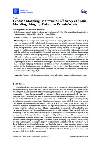
Big Data Cogn. Comput. 2017, 1, 3Big Data Cogn. Comput. 2017, 1, 35 of 145 of a generalizeda generalizedassociationbetweenfoot volumeandexplanatorytwelve explanatoryusedassociationbetweenboardboardfoot volumeper ensedremotelysensedandimagery,and was developedusing aforestrandomforest algorithmderivedfromremotelyimagery,was developedusing a randomalgorithmand theand theRMRSRasterUtility mulations2.2.From aa theoreticaltheoretical standpoint,standpoint, FMFM shouldshould improveimprove processingprocessing efficiencyefficiency byby reducingreducing ssing time and storage space associated with spatial modeling, primarily because it requiresfewer inputinput andandoutputoutputprocesses.processes. However,However, toto justifyjustify thethe useuse ofof FMFM methods,methods, itit isis necessarynecessary ingtimetimeandandstoragestoragespace.space. ToTo evaluateevaluate timeandstoragespaceassociatedwithsixsimulations,we designed, ran, and recorded processing time and storage space associated with six ing(CM)results of those simulations, we compared and contrasted FM with conventional modeling faircomparison.provide a fair oswithinsimulationrangedone onrangedfrom fromone arithmeticoperationto twelvetwelve operationsthat includedarithmetic,logical, conditional,focal,localtype analyses.Countsoperationsthat includedarithmetic,logical, conditional,focal, andlocalandtypeanalyses.Counts howninTable1.Intheinterestofconservingtype of operation included in each model are shown in Table 1. In the interest of conserving space,space, compositefunctionseach modelsof thesearemodelsare not andincludedandhere,definedhere,but, ascompositefunctionsfor eachforof thesenot includeddefinedbut, ldbepresentedinmathematicalform.Eachmodelingin the introduction, each model could be presented in mathematical form. Each modeling scenarioscenariocreateda finalrasterandwas runagainstsix setsrasterdata setsrangingin size fromcreateda finalrasteroutputandoutputwas runagainstsix rasterdatarangingin sizefrom 1,000,000to221,000,000 tototal121,000,000cells(1 mincrementallygrain size), incrementallyincreasingin totalrastersize by121,000,000cells (1 mtotalgrainsize),increasing in totalraster sizeby 2000columns20002000columns2000steprows(addingat each 4step(addingmillioncells ateach step,Figure4). Cellremainedbit depthandrowsandat eachmillioncells4 ateach step,Figure4). Cellbit lscenariosandsimulations.Simulationsconstant as floating type numbers across all scenarios and simulations. Simulations were carriedwereoutcarriedout on a Hewlett‐PackardEliteBookusingan coreI7 Intelquad coreand standardona Hewlett-PackardEliteBook 8740using an8740I7 Intelquadprocessorandprocessorstandard internal5500internal 5500per minute(RPM)harddisk drives (HHD).revolutionsperrevolutionsminute (RPM)hard diskdrives(HHD).These simulations employed stepwise increases in the total number of cells used in the analysis.It is worth noting here that this is a different approach than maintaining a fixed area (i.e., extent) andchanging granularity, gradually moving from coarse to fine resolution and larger numbers of smallerand smaller cells. In this simulation, the algorithm used would produce the same result in both
Big Data Cogn. Comput. 2017, 1, 36 of 14Table 1. The 12 models and their spatial operations used to compare and contrast function modelingand conventional raster modeling in the simulations. Model number (column 1) also indicates the totalnumber of processes performed for a given model. Each of the six simulations included processing all12 models on increasingly large data sets.Model/TotalOperations Arithmetic,Add ( )Type and Number of Spatial OperationsArithmetic,Multiply (*)Logical( )Focal(Mean 7,7)Conditional(True/False)Convolution(Sum, 5,5)Local(Sum )1121131114211- 7 of 14Big Data Cogn.Comput. 2017,1, 35211162211we created12 explanatoryvariables,three predictivemodels,and 1three raster surfacesdepicting722118 estimates3 of BAA, TPA,2 and BFA. 1Average plot1 extent was1 used to extract- andmean plotspectral9321111textural10values in theDNRC studyand was determinedby calculatingaverage limitingdistanceof331111trees dmeasurement(rangingbetween5113311111124311111and 20) and the diameter of each tree measured.Figure 4. Extent, size, and layout of each image within simulations.Figure 4. Extent, size, and layout of each image within simulations.While it would be ideal to directly compare CM with FM for the UNF and DNRC case studies,These simulations employed stepwise increases in the total number of cells used in the analysis.ESRI’s libraries do not have procedures to perform many of the analyses and raster transformationsIt is worth noting here that this is a different approach than maintaining a fixed area (i.e., extent)used in these studies, so CM was not incorporated directly into the analysis. As an alternative toand changing granularity, gradually moving from coarse to fine resolution and larger numbers ofevaluate the time savings associated with using FM in these examples, we used our simulated resultsand estimated the number of individual CM functions required to create GLCM explanatoryvariables and model outputs. Processing time was based on the number of CM functions required toproduce equivalent explanatory variables and predictive surfaces. In many instances, multiple CMfunctions were required to create one explanatory variable or final output. The number of functions
Big Data Cogn. Comput. 2017, 1, 37 of 14smaller and smaller cells. In this simulation, the algorithm used would produce the same result inboth situations. However, some algorithms identify particular structures in an image and try to usecharacteristics like structural patterns and local homogeneity to improve efficiency, especially whenattempting to discern topological relations, potentially using map-based measurements in makingsuch determinations. In these cases, granularity may be important, and comparing the performance ofdifferent approaches would benefit from using both raster size and grain size simulations.To determine the overhead of creating and using a FM, we also conducted a simulation usingfocal mean analyses that varied neighborhood window size across six images. Each iteration ofthe simulation gradually increased the neighborhood window size for the focal mean procedurefrom a 10 by 10 to a 50 by 50 cell neighborhood (in increments of 10 cells) to evaluate the impact ofprocessing more cells within a neighborhood, while holding the image and number of input and outputprocedures constant. Images used in this simulation were the same as in the previous simulation andcontained between 1,000,000 and 121,000,000 total cells. In this scenario, CM and FM techniques wereexpected to show no difference with regard to processing time and storage space using a paired t-testcomparison, and any differences recorded in processing or storage can be attributed to the overheadassociated with creating and using a FM.2.3. Case StudiesTo more fully explore the use of FM to analyze data and create predictive surfaces in realapplications, we evaluated the efficiencies associated with two case studies: (1) a recent study ofthe Uncompahgre National Forest (UNF) in the US state of Colorado [6,29] and (2) a study focusedon the forests of the Montana State Department of Natural Resources and Conservation (DNRC)[unpublished data]. For the UNF study, we used FM, fixed radius cluster plots, and fine resolutionimagery to develop a two-stage classification and estimation procedure that predicts mean values offorest characteristics across 1 million ha at a spatial resolution of 1 m2 . The base data used to create thesepredictions consisted of National Agricultural Imagery Program (NAIP) color infrared (CIR) imagery [30],which contained a total of 10 billion pixels for the extent of the study area. Within this project, we createdno fewer than 365 explanatory raster surfaces, many of which represented a combination of multipleraster functions, as well as 52 predictive models, and 64 predictive surfaces. All of these outputs weregenerated at the extent and spatial resolution of the NAIP imagery (1 m2 , 10 billion pixels).For the DNRC study, we used FM, variable radius plots, and NAIP imagery to predict basal areaper acre (BAA), trees per acre (TPA), and board foot volume per acre (BFA) for more than 2.2 billionpixels ( 0.22 million ha) in northwest Montana USA at the spatial resolution of 1 m2 . In this study,we created 12 explanatory variables, three predictive models, and three raster surfaces depicting meanplot estimates of BAA, TPA, and BFA. Average plot extent was used to extract spectral and texturalvalues in the DNRC study and was determined by calculating average limiting distance of trees withineach plot given the basal area factor used in the field measurement (ranging between 5 and 20) and thediameter of each tree measured.While it would be ideal to directly compare CM with FM for the UNF and DNRC case studies,ESRI’s libraries do not have procedures to perform many of the analyses and raster transformationsused in these studies, so CM was not incorporated directly into the analysis. As an alternative toevaluate the time savings associated with using FM in these examples, we used our simulated resultsand estimated the number of individual CM functions required to create GLCM explanatory variablesand model outputs. Processing time was based on the number of CM functions required to produceequivalent explanatory variables and predictive surfaces. In many instances, multiple CM functionswere required to create one explanatory variable or final output. The number of functions were thenmultiplied by the corresponding propor
Figure 1. A schematic comparing conventional modeling (CM), which employs eager evaluation, to function modeling (FM), which uses lazy evaluation. The conceptual difference between the two modeling techniques is that FM delays evaluation until results are needed and produces results without storing intermediate data sets to disk (green squares).