WIXLIB

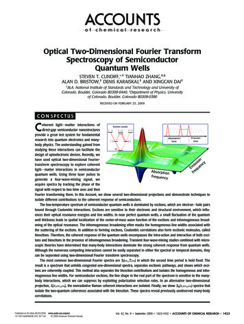
FL44CH18-EckeARI18 November 201115:23Annu. Rev. Fluid Mech. 2012.44:427-451. Downloaded from www.annualreviews.orgAccess provided by University of California - San Diego on 03/17/17. For personal use only.ηα /ην 0; i.e., all the enstrophy goes to small scales to generate the direct enstrophy cascade.This analysis establishes the direction of energy and enstrophy cascades but does not reveal howthe characteristic scales ν and α depend on the physical parameters α and ν.To gain further insight about these relationships, it is convenient to move to Fourier space.Energy at a given wave number k changes at the rate E(k)(9) T (k) F (k) νk2 E(k) α E(k), twhere T(k) represents the rate of energy transfer owing to nonlinear interactions (see Kraichnan& Montgomery 1980), whereas the other terms represent the forcing and dissipation of E(k).Similarly, the nonlinear transfer of enstrophy is given by k2 T (k). The transfer of energy andenstrophy across a scale k defines the fluxes T (k )dk ,(10) E (k) k Z (k) k 2 T (k )dk ,(11)kwith E (0) Z (0) 0 as a consequence of the conservation laws.1/ f ), if the energyIn the inverse-cascade range of wave numbers, kk f (where k fspectrum is dominated by infrared (IR) (small-k) contributions, one has E (k) λk kE(k), whereλk is the characteristic frequency of the distortion of eddies at scale 1/k. Dimensionally, one has kλ2k kmin E( p) p 2 d p, where kmin 1/L is the lowest turbulent wave number, and the upper limitin the integral reflects that scales much smaller than 1/k add incoherently and therefore averageout on scales 1/k.For a scale-free solution E(k) k β , the only expression that gives a scale-independent energyflux E (k) εα is the Kolmogorov solution:E(k) Cεα2/3 k 5/3 ,(12)where C is the dimensionless Kolmogorov constant. Friction induces an IR cutoff at the charεα1/2 α 3/2urms /α, and Equation 12 is expected to holdacteristic friction scale kα 1 αkk f . The extent of this inertial range of scales can be expressedin the range kαin terms of an outer-scale Reynolds number that balances inertial and frictional dissipationReα urms /( f α) α / f k f /kα . The characteristic frequencies in the inverse cascade followthe scaling law λk εα1/3 k2/3 ; therefore, the major contribution to λ2k is from p k, consistent withthe locality assumption.For the direct-cascade range at wave numbers k k f , the enstrophy flux is estimated to beZ (k) λk k3 E(k). A constant enstrophy flux Z (k) ην givesE(k) C ην2/3 k 3 ,(13)where C is another dimensionless constant. Viscous dissipation sets the ultraviolet (large-k) cutoffν 1/2 ην 1/6 with a corresponding Reynolds number Reν u f f /νat a spatial scale kν 1 ν2( f / ν ) . The argument for the direct cascade is, however, not fully consistent. By substitutingEquation 13 into the expression for λ2k , one obtains λk ln(k/kmin ) and thereby a log-k-dependentenstrophy flux. In other words, the assumption of a scale-independent flux is not compatiblewith a pure power-law energy spectrum. A correction to the above argument that restores aconstant Z (k) was proposed by Kraichnan (1971). By looking for a log-corrected spectrum E(k) k 3 [ln(k/kmin )] n , he found that a constant enstrophy flux requires n 1/3 and gives the predictionE(k) C η2/3 k 3 [ln(k/kmin )] 1/3 .(14)www.annualreviews.org Two-Dimensional Turbulence431

ARI18 November 201115:23This correction has a weak point in the assumption of locality. In the expression in Equation 14,k. Therefore, the situation is quite different from aλ2k is IR dominated by wave numbers pKolmogorov 5/3 spectrum (in both two and three dimensions) in which transfer rates are localin k. Rather, it is similar to the stirring of a passive scalar in the Batchelor regime (Batchelor 1959)in which the dominant straining comes from the largest scales. The analogy with passive scalarsbecomes stronger in the presence of friction: The inclusion of a damping term in Equation 1 has adramatic effect on the direct enstrophy cascade in which it changes the exponent of the spectrum,as discussed in Section 4.3.For an energy spectrum of the form E(k) k β , one expects power-law scaling in r for the second-order velocity structure function. Indeed, for any λ, we have S2 (λr) 4 0 dkE(k)[1 J0 (kλr)] λβ 1 S2 (r), which implies S2 (r) r β 1 . This argument is consistent only if theintegral over k is not IR or ultraviolet divergent (i.e., is dominated by local contributions). Takinginto account the asymptotic behaviors of J0 (x), one obtains the so-called locality condition forconvergence: 1 β 3. Under this condition, E(k) and S2 (r) contain the same scaling information.(L)Inof the inverse cascade, the prediction is therefore S2 (r) C2 ε2/3 r 2/3 , with C2 the case3π/[25/3 2 (4/3)]C 2.15C. For the direct cascade, Equation 13 gives S2 (r) r 2 , but this isat the border of the IR locality condition (β 3). Therefore, the velocity structure functions aredominated by the largest scales and are not informative about the small-scale turbulent components(the same r2 behavior is expected for any spectrum with β 3). More information is obtainedby looking at the statistics of small-scale-dominated quantities, the most natural being structurefunctions of vorticity.Constant energy and enstrophy fluxes in the respective inertial ranges imply exact relations forthe third-order structure function (see Frisch 1995, Bernard 1999, Lindborg 1999, Yakhot 1999).For homogeneous, isotropic conditions over the range of scales in the inverse cascade (r f ),one has3(L)S3 (r) [δu (r)]3 3 δu (r)[δu (r)]2 ε I r,(15)2which is the 2D equivalent of the 3D Kolmogorov 4/5 law. In the range of scales of the directenstrophy cascade (rf ), the prediction isAnnu. Rev. Fluid Mech. 2012.44:427-451. Downloaded from www.annualreviews.orgAccess provided by University of California - San Diego on 03/17/17. For personal use only.FL44CH18-Ecke(L)S3 (r) 1ηI r 3,8(16)which can also be written for the mixed velocity-vorticity structure function, representing theenstrophy flux, as δu (r)[δω(r)]2 2η I r.(17)Assuming self-similarity, Equation 15 leads to the scaling exponent of 1/3 for velocity fluctuationsin the inverse cascade and therefore to a Kolmogorov prediction for the exponents of the velocitystructure functions Sn (r) r ζn with ζn n/3. At variance with the 3D case in which deviationsare found (Frisch 1995), this mean field prediction is supported by simulations and experimentsin the inverse cascade of 2D turbulence.3. METHODS AND APPROACHESIn this section, we discuss general methods and approaches for experimental realizations and numerical simulations of 2D turbulence. Physical fluid systems are intrinsically 3D. By constrainingmotion in one spatial direction, however, one can produce fluid motion that is approximately 2D.There are numerous ways to apply such a constraint with quite different resultant 3D perturbations. There are two main types of constraints: (a) body forces including stratification, rotation,432Boffetta·Ecke

Annu. Rev. Fluid Mech. 2012.44:427-451. Downloaded from www.annualreviews.orgAccess provided by University of California - San Diego on 03/17/17. For personal use only.FL44CH18-EckeARI18 November 201115:23and magnetic fields and (b) geometric anisotropy in which the length scale in one direction ismuch smaller than in the other two. Both constraints are important in geophysical and astrophysical systems. For example, one can treat some aspects of motion in atmospheres or oceans asapproximately 2D because of the much smaller depth of the atmosphere (ocean), 10 km, relativeto lateral global scales, 103 –104 km.We focus here on two experimental realizations of 2D turbulence that have been widely utilized,namely thin electrically conducting layers driven by a combination of a fixed array of magnetswith an applied electrical current and soap films flowing under the force of gravity. We do notdiscuss other realizations of 2D turbulence using rotation, stratification, and magnet fields. In alllaboratory realizations of 2D turbulence, the flows are damped by coupling to boundaries. We treatthis as a linear frictional damping proportional to the velocity with coefficient α as in Equation 1with a form discussed below for each system. A nondimensional measure of damping, α α/ωrms(or, equivalently, a Reynolds number Reα 1/α ), allows one to compare the relative importanceof friction among different systems. In the cases considered here, the fluid equations governingthe quasi-2D flows have not been unambiguously demonstrated to satisfy the 2D Navier-Stokesequation (see Couder et al. 1989, Paret et al. 1997, Chomaz 2001, Rivera & Wu 2002), but themapping is not an unreasonable one. Our main focus here is on experiments in which one canmeasure the full velocity field and thereby extract information that elucidates the physics of 2Dturbulence in a complete way. An important point for experiments is that the degree to which theresults for idealized 2D turbulence apply to the quasi-2D systems is a measure of the applicabilityof these predictions to 3D systems such as Earth or planetary atmospheres.As opposed to laboratory experiments, truly 2D flows are easily realizable in silico; therefore, direct numerical simulation (DNS) is one of the most powerful methods for studying 2Dturbulence (see Figure 1). Lilly (1969) first attempted the simulation of 2D turbulence using afinite-difference scheme on a 64 64 grid to study both the cascades predicted by Kraichnan.This early attempt was not successful in observing coexisting cascades as much higher resolutionis actually needed (Boffetta 2007).Many simulations of 2D turbulence do not integrate Equation 2 but instead consider a variantin which viscous dissipation and friction are replaced by higher-order terms ( 1) p 1 ν p 2 p ω and( 1)q 1 αq 2q ω, respectively. The motivation for the use of hyperviscosity ( p 1) and hypofriction (q 0) is to reduce the range of scales over which dissipative terms contribute substantially,thereby extending the inertial range for a given spatial resolution. Recent studies (Lamorgese et al.2005, Frisch et al. 2008, Bos & Bertoglio 2009) suggest that these modified dissipation approachescan seriously affect the statistics at the transition between inertial and dissipative scales.Energy and enstrophy input for DNS are usually implemented numerically using a Gaussianstochastic forcing with zero mean and correlation function f (x , t ) f (x, t) F (x x, t t). Thespatial dependence of F is chosen to restrict the injection to a range of scales around f , whereasthe temporal component is usually white noise, F (x x, t t) F (r)δ(t t ), which fixes a priorithe mean enstrophy (and energy) input as η I F (0)/2 (Novikov 1965).Experiments on 2D turbulence have external forcing that is fixed in space, either by a grid,as in decaying turbulence in a soap film channel, or by the fixed array of magnets for horizontalsoap films and stratified layers. Standard magnet configurations include (a) a pseudo-random setof positions with a mean separation distance (Williams et al. 1997, Voth et al. 2003, Twardoset al. 2008), (b) block random forcing in which small magnets of the same polarity are arranged inlarger blocks (Paret et al. 1999, Boffetta et al. 2005) in an attempt to produce a random large-scaleforcing (this scheme results in energy injection at the scale of the magnet as well as at the blockscale), (c) Kolmogorov flow using strip magnets (Rivera & Wu 2000) or lines of magnets in whichcase there is a weak perturbation on pure parallel shear flow, and (d ) square-array forcing.www.annualreviews.org Two-Dimensional Turbulence433

FL44CH18-EckeARI18 November 2011Annu. Rev. Fluid Mech. 2012.44:427-451. Downloaded from www.annualreviews.orgAccess provided by University of California - San Diego on 03/17/17. For personal use only.a ω15:23b ωc ωsNegative0d ZPositiveVorticity or enstrophy fluxFigure 2The decomposition of a soap-film vorticity field using the filter approach to obtain the enstrophy flux: (a) unfiltered vorticity ω,(b) filtered large-scale vorticity ω , (c) small-scale vorticity ωs ω ω , and (d ) enstrophy flux Z .Experimentally, one has more options for temporal forcing. The electric current can be sinusoidally periodic or square-wave periodic or it can be telegraph noise, i.e., with constant amplitudebut varying intervals of positive and negative polarity of the current with zero mean. The optimal temporal forcing is not well understood, but some general observations can be noted: If thefrequency is too high, the forcing does not couple well with the fluid degrees of freedom, andlittle net energy is injected into the fluid. The optimal transfer of energy occurs for direct-currentforcing, but there is preferential buildup at the injection scale and possible coupling to large-scaleinhomogeneities in the forcing (e.g., magnet arrangement, layer height). A systematic study offorcing has not been performed for experimental 2D turbulence.An analysis method that has proved useful for both experimental (Rivera et al. 2003, Chen et al.2006) and numerical (Xiao et al. 2009) data is based on the filter approach, the basis for large-eddysimulations. This methodology can be applied either to the velocity field to yield information aboutthe energy flux or to the vorticity field to obtain the enstrophy flux. We consider the vorticityhere for simplicity, with details found elsewhere (Xiao et al. 2009). The vorticity field ω(x, y) is22smoothed with a low-pass filter with cutoff , e.g., G (r) e r /(2 ) , to create a filtered vorticityfield ω̄ . One obtains an equation for the large-scale enstrophy : t (r, t) · K (r, t) Z (r, t),(18)where K is the space transport of enstrophy, Z (r, t) ω̄ (r, t)·σ (r, t) is the enstrophy flux outof large scales greater than into small-scale modes, and σ (uω) ū ω̄ is the space transport ofvorticity owing to the eliminated small-scale turbulence. The exciting aspect of this filter methodis that one obtains scale-to-scale information as a function of real space coordinates. An exampleof the filter approach drawn from experimental soap-film data (Rivera et al. 2003) is shown inFigure 2 in which the vorticity field ω is decomposed into the filtered large-scale field ω̄ and thesmall-scale field ω̄s ω ω̄ . The resultant Z shows the physical space distribution of enstrophyflux. This representation provides an opportunity to quantitatively test physical mechanisms ofthe direct enstrophy process (Rivera et al. 2003) or the inverse energy cascade using the filteredenergy flux (Chen et al. 2006, Xiao et al. 2009).434Boffetta·Ecke

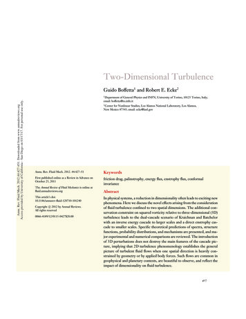
FL44CH18-EckeARI18 November 201115:23Annu. Rev. Fluid Mech. 2012.44:427-451. Downloaded from www.annualreviews.orgAccess provided by University of California - San Diego on 03/17/17. For personal use only.3.1. Electromagnetically Forced Conducting Fluid LayersAn effective way to induce fluid motion in a highly controlled manner in thin layers of conductingfluids is to arrange an array of magnets beneath the layer and to apply a spatially uniform currentin the plane of that layer. The resulting Lorentz force induces horizontal motion. A schematicillustration of an electromagnetic layer (EML) experiment is shown in Figure 3a. The flexibilityof the placement of the magnets and of the application of different time sequences of the electriccurrent makes this system amenable to experimental study. In particular, there is no mean flow,and because of the strong two-dimensionality of the flow, particles are straightforward to trackdirectly, and velocity fields are obtained using particle tracking velocimetry (PTV) [or, withless fidelity, particle image velocimetry (PIV)]. Examples of such reconstructions are shown inFigure 3b,c. An advantage of EML systems is approximately incompressible Newtonian fluidflow for modest forcing with well-understood and controllable boundary drag, which makes themsuitable for studies of the inverse energy cascade and for Lagrangian measurements. However, theReynolds numbers of the flow are limited because vigorous forcing induces compressibility effects(or thickness variations for soap films), including surface waves, and may cause Joule heating ofthe layers at higher currents. Finally, the relatively large thickness of salt layers makes the directcascade hard to resolve as the generation of fine vortex filaments is limited by the layer thickness.There have been several manifestations of EML systems using different fluids and magneticconfigurations: a layer of mercury over an array of source/sinks of electric current with a largescale, constant magnetic field; a layer of saltwater with and without buffering layers to reducebottom drag; and a soap film made electrically conducting by the addition of salt. For each systemwe describe the typical ranges of parameters, including drag coefficients and Reynolds numbers.One of the first experiments on 2D turbulence was done by Sommeria (1986) in a h 2-cmdeep layer of mercury with lateral dimensions L 12 cm and aspect ratio L/ h 6. A constantfield magnet (0.1–1 Tesla) generated a Hartmann layer δ H between 30 and 250 μm. A square arrayof alternating sources of electric current induced vorticity on a forcing scale f 1 cm. Electricpotential probes measured the local velocity with high accuracy. Owing to the small kinematicviscosity of mercury, ν 10 3 cm2 s 1 , the injection-scale Reynolds number Reν urms f /νaElectricalcontactbSaltwaterBuffer layercElectricalcontactMagnet arrayCurrent sourceNegative0PositiveVorticityFigure 3(a) Schematic illustration of an electromagnetically forced thin layer system with an immisciblenonconducting bottom fluid and an upper salt solution. Differences in the apparatus depend on experimentaldetails, e.g., mercury with a thin Hartmann layer (Sommeria 1986) or a miscible bottom salt solution with apure-water upper layer (Paret & Tabeling 1997). Examples of 2D field measurements in electromagneticlayers include (b) a vorticity field in a stationary inverse cascade by Paret & Tabeling (1997) and (c) particletrajectories of a velocity field for stratified immiscible layers described by Rivera & Ecke (2005) (false color).c 1997 by the American Physical Society.Panel b reproduced by permission, copyright www.annualreviews.org Two-Dimensional Turbulence435

ARI18 November 201115:23reached 104 , whereas the outer-scale Reynolds number Reα urms /( f α) was set by frictionaldamping so that Reα 5. Similarly, 1 α 10, reflecting the large damping of the thinHartmann layer.The most widely studied system for 2D turbulence is a single saltwater layer with thickness0.2 h 1 cm and L 20 cm (Cardoso et al. 1994, Bondarenko et al. 2002) or two layersof fluid, either miscible (Marteau et al. 1995) or immiscible (Rivera & Ecke 2005) combinations,with similar thicknesses. The aspect ratio L/ h 100 is considerable although L/ f 20 forf 1 cm. Boundary drag is an important feature of this system and is relatively easy to calculate.For a single layer, the rigid boundary condition on the bottom and free-surface boundary at thetop imply α νπ 2 /(2h 2 ) (Dolzhanskii et al. 1992). With typical values of h 0.3 cm and ν 0.01cm2 s 1 , one obtains α 0.5 s 1 . Using the miscible double-layer configuration—top water layerover bottom saltwater lay

servation constraint on squared vorticity relative to three-dimensional (3D) turbulence leads to the dual-cascade scenario of Kraichnan and Batchelor with an inverse energy cascade to larger scales and a direct enstrophy cas-cade to smaller scales. Specific theoretical predictions of spectra, structure