Transcription
H EIDELBERG U NIVERSITYD EPARTMENT OF P HYSICS AND A STRONOMYTheoretical Statistical Physicsipts by UlrichrcsScreid esivertyHearzhwLectuProf. Ulrich SchwarzWinter term 2020/21Last update: February 16, 2021lb e rg U ni
ForewordThis script is written for the course Theoretical Statistical Physics which is one of thecore courses for the master studies of physics at Heidelberg University, although inpractise it is also attended by many bachelor students from the 5th semester. I have beengiving this course several times before, namely in the winter terms of 2012, 2015, 2017and 2020, and it is my experience that a script helps to correct the unavoidable errorsmade at the blackboard, to solidify the new knowledge through a coherent presentationand to prepare for the final exam. There exist many very good textbooks on statisticalphysics and the purpose of this script is soley to document my personal choice of therelevant material.Statistical physics provides the basis for many important parts of physics, includingatomic and molecular physics, solid state physics, soft matter physics, biophysics, astrophysics, environmental and socioeconomic physics. For example, you cannot understand the greenhouse effect or the cosmic microwave background without the Planckformula for the statistics of photons at a given temperature (black body radiation) orthe electrical conduction of solids without the concept of a Fermi sphere (the groundstate of a fluid of electrons at low temperature). Equally important, however, statisticalphysics provide the basis for our understanding of phase transitions, which are truelycollective effects and often do not depend much on microscopic details. As you willlearn in this course, at the heart of statistical physics is the art of counting, which is formalized in the concept of a partition sum. The details of how this has to be done indifferent systems can be quite challenging, and thus it should not come as a surprisethat statistical physics is still a very active research area, continuously expanding intonew applications and developing new methods.Several guiding principles and helpful books determined the design of this course.First I completely agree with Josef Honerkamp who in his book Statistical Physics notesthat statistical physics is much more than statistical mechanics. A similar notion is expressed by James Sethna in his book Entropy, Order Parameters, and Complexity. Indeedstatistical physics teaches us how to think about the world in terms of probabilities.This is particularly relevant when one deals with complex systems and real world data.Therefore applications of statistical physics can also be found in data-intensive researchareas such as astrophysics, environmental physics, biophysics, socioeconophysics andphysics of information (including machine learning). As instructive examples, considerthe models for the spread of rumours or viruses on networks, or the algorithms used forsegmentation and object recognition in image processing. If you investigate how thesemodels work, you will realize that they often relate to the Ising model for ferromagnets,arguably the most important model of statistical physics and an important subject forthis course.
Second a course on statistical physics certainly has to make the connection to thermodynamics. Thermodynamics can be quite cubersome and hard to digest at times, soa pedagogical approach is highly appreciated by most students. Here I am stronglymotivated by the axiomatic and geometrical approach to thermodynamics as layed outin the beautiful book Thermodynamics and an introduction to Thermostatistics by HerbertCallen. Historically thermodynamics developed as a phenomenological theory of heattransfer, but when being approached from the axiomatic and geometrical side, it becomes the convincing and universal theory that it actually is. The book by Callen alsodraws heavily on the work by Edwin Jaynes on the relationship between statisticalphysics and information theory as pioneered by Claude Shannon. Although somehowdebated, this link shows once again that statistical physics is more than statistical mechanics. Information theory provides very helpful insight into the concept of entropy,which is the cornerstone of statistical mechanics. Recently this area has been revivedby the advent of stochastic thermodynamics, which shows that entropy is not only anensemble property, but can also be defined for single trajectories.Third a comprehensive course on statistical physics should also include some numerical component, because modern statistical physics cannot be practised without computational approaches, as again nicely argued by Josef Honerkamp and James Sethna.Moreover statistical physics is much more than thermodynamic equilibrium and iftime permits, a course on statistical physics should also cover some aspects of nonequilibrium physics, for example the exciting recent developments in stochastic thermodynamics. Although it is hard to fit all of these aspects into a one-semester course,some of them are included here.Together, these considerations might explain the structure of this script. We start withan introduction to the concepts of probability theory, which should be useful also inother contexts than only statistical mechanics. We then introduce the fundamental postulate of equilibrium physics, namely that each microstate is equally probable, leadingto the microcanonical ensemble and the principle of maximal entropy. We then discussthe canoncial and grandcanonical ensembles, when reservoirs exist for exchange of heatand particle number, respectively. We then apply these concepts to quantum fluids, inparticular the Fermi fluid (e.g. electrons in a solid) and the Bose gas (e.g. black bodyradiation with photons or the Debye model for crystal vibrations). These are interacting systems, but this is accounted for by the right way to count, not by investigatingdirect interactions. Yet, here we encounter our first phase transition, the Bose-Einsteincondensation. We then introduce the concept of phase transitions emerging from directinteractions through the example of the Ising model. In particular, it is here that weintroduce one of the most important advances of theoretical physics of the 20th century, namely the renormalization group. We then continue to discuss phase transitions,now for complex fluids, starting with the van der Waals fluid and the virial expansion. We close with a discussion of thermodynamics, from which we see that statisticalphysics and thermodynamics essentially use the same formal structure, but that theycomplement each other in a unique manner: statistical physics focuses on the emergence of macroscopic properties from microscopic mechanisms, and thermodynamicson the macroscopic principles that necessarily have to be valid in the thermodynamic
limit of very large system size, independent of microscopic details.Finally one should note some subjects which are not covered in the script due to spacereasons. We do not cover kinetic and transport theories, which would also includethe Boltzmann equation. The very important subject of fluctuations and correlations(including the fluctuation-dissipation theorem) is mentioned only in passing. We alsocannot treat much out-of-equilibrium physics here, in particular we do not cover GreenKubo relations, Onsager’s reciprocity theorem, Kramers-Krönig relations or linear response theory. From the subject side, we will not have time to cover such interesting subjects as liquid crystals, percolation, disordered and glassy systems (includingthe replica method), nucleation, coarsening and Ostwald ripening, or the dynamics ofchemical reactions and populations.Heidelberg, winter term 2020/21Ulrich Schwarz
Contents1 Introduction to probability theory1.1 Probability in physics . . . . . . . . . . . . . . . . . .1.2 Frequentist approach . . . . . . . . . . . . . . . . . .1.3 Axiomatic approach . . . . . . . . . . . . . . . . . .1.4 Continuous distributions and distribution function1.5 Joint, marginal and conditional probabilities . . . .1.6 Expectation and covariance . . . . . . . . . . . . . .1.7 Binomial distribution . . . . . . . . . . . . . . . . . .1.8 Gauss distribution . . . . . . . . . . . . . . . . . . .1.9 Poisson distribution . . . . . . . . . . . . . . . . . . .1.10 Random walks . . . . . . . . . . . . . . . . . . . . . .1.11 Computation with random variables . . . . . . . . .1.12 Addition of random variables . . . . . . . . . . . . .1.13 Information entropy . . . . . . . . . . . . . . . . . .1112449101518192325282 The microcanonical ensemble2.1 Thermodynamic equilibrium . . . . . . .2.2 Micro- and macrostates . . . . . . . . . . .2.3 Density of states . . . . . . . . . . . . . . .2.4 The fundamental postulate . . . . . . . .2.5 Equilibrium conditions . . . . . . . . . . .2.6 Equations of state for ideal gas . . . . . .2.7 Two-state system . . . . . . . . . . . . . .2.8 Einstein model for specific heat of a solid2.9 Entropic elasticity of polymers . . . . . .2.10 Statistical deviation from average . . . . .2.11 Foundation of the fundamental postulate.3333343537414647505355573 The canonical ensemble3.1 Boltzmann distribution .3.2 Free energy . . . . . . . .3.3 Non-interacting systems3.4 Equipartition theorem .3.5 Molecular gases . . . . .3.6 Specific heat of a solid .3.7 Black body radiation . .6262646772758086.
4 The grandcanonical ensemble4.1 Probability distribution . . . . . . . .4.2 Grandcanonical potential . . . . . .4.3 Fluctuations . . . . . . . . . . . . . .4.4 Ideal gas . . . . . . . . . . . . . . . .4.5 Molecular adsorption onto a surface4.6 Chemical reactions . . . . . . . . . .939394959697985 Quantum fluids5.1 Fermions versus bosons . . . . . . . .5.2 Calculating with occupation numbers5.3 The ideal Fermi fluid . . . . . . . . . .5.4 The ideal Bose fluid . . . . . . . . . . .5.5 Classical limit . . . . . . . . . . . . . .1011011061071151226 Ising model6.1 Definition . . . . . . . . . . . . . . . . . . . . . . . . .6.2 The 1d Ising model . . . . . . . . . . . . . . . . . . . .6.3 Transfer matrix . . . . . . . . . . . . . . . . . . . . . .6.4 Renormalization of the Ising chain . . . . . . . . . . .6.5 Renormalization of the 2d Ising model . . . . . . . . .6.6 The Peierls argument . . . . . . . . . . . . . . . . . . .6.7 The 2d Ising model . . . . . . . . . . . . . . . . . . . .6.8 Perturbation theory . . . . . . . . . . . . . . . . . . . .6.9 Mean field theory for the Ising model . . . . . . . . .6.10 Monte Carlo computer simulations of the Ising model.1241241281311361401411441471481517 Classical fluids7.1 Virial expansion . . . . . . .7.2 Second virial coefficient . .7.3 Maxwell construction . . . .7.4 Fluid-solid phase transition7.5 Distribution functions . . .1531531561611651678 Thermodynamics8.1 Axiomatic structure . . . . . . . . . . . . . . . . . . . . . . .8.2 Variational principles . . . . . . . . . . . . . . . . . . . . . .8.3 Euler and Gibbs-Duhem relations . . . . . . . . . . . . . . .8.4 Thermodynamic potentials and Legendre transformations8.5 Maxwell relations . . . . . . . . . . . . . . . . . . . . . . . .8.6 Process-dependance of work and heat . . . . . . . . . . . .8.7 Reversible and irreversible processes . . . . . . . . . . . . .8.8 Thermodynamic engines . . . . . . . . . . . . . . . . . . . .8.9 Chemical reactions . . . . . . . . . . . . . . . . . . . . . . .170170171174176179182186189194.
9 Non-equilibrium statistical physics19910 Appendix: some useful relations between partial derivatives202
1 Introduction to probability theory1.1 Probability in physicsClassical physics (classical mechanics and electrodynamics) is deterministic, that meansthe governing equations (Newton’s and Maxwell’s equations, respectively) are differential equations that have a unique solution once we know the initial conditions (andboundary conditions for the case of Maxwell’s equations, which are partial differentialequations). Quantum mechanics of course introduces probability into physics in theform of the statistical (Kopenhagen) interpretation, that is experiments lead to the collapse of the wavefunction with probabilistic outcomes, but still we solve a deterministicdifferential equation (Schrödinger’s equation for the wavefunction) and then probability for the outcome follows as the squared modulus of the complex wavefunction.In marked contrast, statistical physics directly brings the concept of probability intophysics. Now the central concept is to calculate the probability of a certain macroscopicstate, thus probability is not a derived quantity, but the most elementary concept. Forexample, in the canonical ensemble the relevant statistics will be the Boltzmann distribution. Therefore we start our course on statistical physics with an introductioninto probability theory. Later of course we have to ask how the probabilistic natureof statistical physics emerges from more microscopic descriptions, and we will see thatboth classical and quantum mechanics provide some justification for this (deterministicchaos and thermalization of the wavefunction, respectively).1.2 Frequentist approachThe history of probability theory is long and twisted. Yet everybody has an intuitivenotion of probability that is related to frequencies of certain outcomes. We start witha simple example (throwing dice) to illustrate what this means and what one wouldexpect from a theory of probability. Possible outcomes for a die are {1, 2, 3, 4, 5, 6}. ForN throws the event {i } occurs Ni times. We then identify the probability pi for event{i } with its frequency:pi # favorable outcomesN i# possible outcomesNFor an ideal die we expect pi around 167 times.16in the limit N 0.167. Hence for 1000 throws {6} should occur1
We first note that our definition is normalized:6 Ni N1/N i 16 pi 1i 1We next consider events that are not directly an experimental outcome, but a morecomplicated question to ask about the system. E.g. what is the probability to get anodd outcome?podd # favorable outcomesN N3 N5 1 p1 p3 p5# possible outcomesNsum rule: summation of probabilities for simultaneous disjunct eventsWhat is the probability to get twice {6} when throwing two times? We first throw Ntimes and find N6 times a 6. We then throw M times and find M6 times a 6. Thus wecountN6 · M6N6 M61# favorable outcomesp66 · p6 · p6 # possible outcomesN·MN M36 product rule: multiplication of probabilities for subsequent independent eventsFinally we note that we could either throw N dice at once or the same die N times - theresult should be the same ergodic hypothesis of statistical physics: ensemble average time averageIdentifying probability with frequency is called the classical or frequentist interpretationof probability. There are two problems with this. First there are some examples forwhich naive expectations of this kind fail and a more rigorous theory is required. Second there are many instances in which an experiment cannot be repeated. Consider e.g.the statistical distribution of galaxy sizes in the universe, for which we have only onerealization in our hands. In order to address these problems, the concept of probabilitycan be approached by an axiomatic approach.1.3 Axiomatic approachAbove we described an empirical approach to measure probability for the dice throwing experiment and this sharpened our intuition what we expect from a theory of probability. We now construct a mathematical theory of probability by introducing an axiomatic system (Kolmogorov 1933). It has been shown that this approach allows to describe also complex systems without generating contradictions1 .Let Ω {ωi } be the set of elementary events. The complete set of possible events isthe event space B defined by:1 Foran introduction into probability theory, we recommend Josef Honerkamp, Stochastische DynamischeSysteme, VCH 1990; and Geoffrey Grimmett and Dominic Welsh, Probability: an introduction, 2nd edition2014, Oxford University Press.2
1Ω B2if A B , then A B3if A1 , A2 , · · · B , then i 1 Ai BBy setting all Ai with i larger than a certain value to empty sets, the last point includesunions of a finite number of sets. We see that the event space is closed under the operations of taking complements and countable unions. This concept is also known asσ-algebra. In our case we actually have a Borel-algebra, because the σ-algebra is generated by a topology. The most important point is that we have to avoid non-countableunions, because this might lead to pathological situations of the nature of the BanachTarski paradoxon (which states that a sphere can be disassembled into points and thatthey then can be reassembled into two spheres because the set of real numbers is noncountable).Corollaries1 B2A B A B BExamples1Ω {1, ., 6} for the ideal die. This set of elementary events is complete andSdisjunct (ωi ω j if i 6 j, 6i 1 ωi Ω ). This event space is discrete.2All intervals on the real axis, including points and semi-infinite intervals like x λ. Here x could be the position of a particle. This event space is continuous.We now introduce the concept of probability. For each event A in the event space B weassign a real number p( A), such that1p( A) 02p(Ω) 13p(Si A BAi ) i p ( Ai )if Ai A j for i 6 jNote that the last assumption is the sum rule. Kolmogorov showed that these rules aresufficient for a consistent theory of probability.3
Corollaries1p( ) 02p( A) p( A) p(Ω) 13Consider A1 , A2 B : p( A) 1 p( A) 0 p( A) 1p ( A1 ) p ( A1 A2 ) p ( A1 A2 ) {z }: C1p ( A2 ) p ( A2 A1 ) p ( A2 A1 ) {z }: C2 p( A1 ) p( A2 ) p(C1 ) p(C2 ) 2p( A1 A2 ) p ( A1 A2 ) p ( A1 A2 )p ( A1 A2 ) p ( A1 ) p ( A2 ) p ( A1 A2 )1.4 Continuous distributions and distribution functionConsider the event space containing the intervals and points on the real axis. p( x λ)is the probability that x is smaller or equal to a given λ (eg the position of a particle in1D):P(λ) : p( x λ) cumulative distribution functionIf P(λ) is differentiable, thenP(λ) Z λ p( x )dxwheredP(λ)probability density or distribution functiondλRxWe now can write the probability for x [ x1 , x2 ] as x12 p( x )dx. With x2 x1 dx1 ,we can approximate the integral by a product and thus find that p( x1 )dx1 is the probability to have x [ x1 , x1 dx1 ]. Thus p( x ) is the probability density and p( x )dx is theprobability to find a value around x. Note that the physical dimension of p( x ) is 1/m,because you still have to integrate to get the probability.p(λ) 1.5 Joint, marginal and conditional probabilitiesA multidimensional distribution x ( x1 , .xn ) is called a multivariate distribution, ifp( x ) dx1 . dxn is the probability for xi [ xi , xi dxi ]We also speak of a joint distribution. Note that in principle we have to distinguishbetween the random variable and its realization, but here we are a bit sloppy and donot show this difference in the notation.4
Examples1A classical system with one particle in 3D with position and momentum vectorshas six degrees of freedom, thus we deal with the probability distribution p( q, p).For N particles, we have 6N variables.2We measure the probability p( a, i ) for a person to have a certain age a and a certainincome i. Then we can ask questions about possible correlations between age andincome.3Consider a collection of apples (a) and oranges (o) distributed over two boxes (leftl and right r). We then have a discrete joint probability distribution p( F, B) whereF a, o is fruits and B l, r is boxes.Marginal probability: now we are interested only in the probability for a subset of allvariables, e.g. of x1 :Zp ( x1 ) dx2 . dxn p( x )is the probability for x1 [ x1 , x1 dx1 ] independent of the outcome for x2 , ., xn .Examples1We integrate out the momentum degrees of freedom to focus on the positions.2We integrate p( a, i ) over i to get the age structure of our social network.3We sum over the two boxes to get the probability to have an orangep(o ) p(o, l ) p(o, r )This example shows nicely that the definition of the marginal probability essentially implements the sum rule.Conditional probability: we start with the joint probability and then calculate the marginalones. From there we define the conditional ones. Consider two events A, B B . Theconditional probability for A given B, p( A B), is defined byp( A, B) {z }joint probability p( A B) {z }·p( B) {z }conditional probability for A given B marginal probability for BThus the definition of the conditional probability essentially introduces the productrule.5
ExampleConsider a fair die and the events A {2} and B {2, 4, 6}.p( A B) p( A)1p( A, B) p( B)p( B)3p( B A) p( A, B)p( A) 1p( A)p( A)Statistical independence: p( A1 A2 ) p( A1 )A1 is independent of A2 p ( A1 , A2 ) p ( A1 A2 ) p ( A2 ) p ( A1 ) p ( A2 )Thus we get the product rule (multiplication of probabilities) that we expect for independent measurements, compare the example of throwing dice discussed above. Wealso see thatp ( A1 , A2 ) p ( A2 A1 ) p ( A2 )p ( A1 )Statistic independence is mutual.Bayes’ theorem: p( A, B) p( A B) · p( B) p( B, A) p( B A) · p( A)p( B A) p( A B) · p( B)p( A B) · p( B) p( A) B0 p ( A B 0 ) · p ( B 0 )Bayes’ theoremwhere for the second form we have used the sum rule. Despite of its simplicity, this formula named after Thomas Bayes (1701-1761) is of extremely large practical relevance. Itallows to ask questions about the data that are not directly accessible by measurements.Examples1Consider again the fruits (F a, o) in the boxes (B l, r). We assume that leftand right are selected with probabilites p(l ) 4/10 and p(r ) 6/10 (they sumto 1 as they should). We next write down the known conditional probabilities bynoting that there are two apples and six oranges in the left box and three applesand one orange in the right box:p( a l ) 1/4, p( o l ) 3/4, p( a r ) 3/4, p( o r ) 1/4We now ask: what is the probability of choosing an apple ?p( a) p( a l ) p(l ) p( a r ) p(r ) 11/20Note that the result is not 5/12 that we would get if there was no bias in choosingboxes. The probability of choosing an orange isp(o ) 1 p( a) 9/206
We next ask a more complicated question: if we have selected an orange, what isthe probability that it did come from the left box ? The answer follows by writingdown the corresponding conditional probability:p( l o ) p( o l ) p(l ) 2/3p(o )Thereforep( r o ) 1 2/3 1/3Above we have formulated the probability p( F B) for the fruit conditioned onthe box. We now have reverted this relation to get the probability p( B F ) for thebox conditioned on the fruit. Our prior probability for the left box was p(l ) 4/10 0.5. Our posterior probability for the left box, now that we know thatwe have an orange, is p( l o ) 2/3 0.5. Thus the additional information hasreverted the bias for the two boxes.2We discuss the statistics of medical testing. Imagine a test for an infection withthe new Corona virus Sars-CoV-2. The standard test is based on the polymerasechain reaction (PCR), but now there new tests that are cheaper and faster, butnot as reliable (e.g. the LAMP-test from ZMBH Heidelberg or the rapid antigentest by Roche). At any rate, such a test always has two potential errors: falsepositives (test is positive, but patient is not infected) and false negatives (test isnegative, but patient is infected). We have to quantify these uncertainties. Let’sassume that the probability that the test is positive if someone is infected is 0.95 (sothe probability for false negatives is 0.05) and that the probability that the test ispositive if someone is not infected is 0.01 (false positives). Actually these numbersare quite realistic for antigen tests against Sars-CoV-2 (PCR-tests are much morereliable).Let A be the event that someone is infected and B the event that someone is testedpositive. Our two statements on the uncertainties are then conditional probabilities:p( B A) 0.95, p( B Ā) 0.01 .We now ask what is the probability p( A B) that someone is infected if the test waspositive. As explained above, this question corresponds to the kind of change ofviewpoint that is described by Bayes’ theorem. We will answer this question asa function of p( A) x, because the answer will depend on which fraction of thepopulation is infected.According to Bayes’ theorem, the conditional probability p( A B) is determinedbyp( B A) xp( B A) xp( A B) .(1.1)p( B)p( B A) x p( B Ā) p( Ā)7
Using x p( Ā) 1, we getp( A B) p( B A) x h[ p( B A) p( B Ā)] x p( B Ā)1 xip( B Ā)p( B A)x p( B Ā)p( B A).(1.2)Introducing the ratio of false positive test results to correctly positive ones, c : p( B Ā)/p( B A), we have our final resultp( A B) x.[1 c ] x c(1.3)Thus the probability p( A B) that someone is in fact infected when tested positivevanishes for x 0, increases linearly with x for x c and eventually saturatesat p( A B) 1 as x 1. This type of saturation behaviour is very common inmany applications, e.g. for adsorption to a surface (Langmuir isotherm) or in theMichaelis-Menten law for enzyme kinetics.Putting in the numbers from above gives c 0.01 1. Therefore we can replacethe expression for p( A B) from above byp( A B) x.c x(1.4)For a representative x-value below c, we take x 1/1000 (one out of 1000 peopleis infected). Then p( A B) 0.1 and the probability to be infected if the test is positive is surprisingly small. It only becomes 1/2 if x c (one out of 100 people isinfected). Thus the test only becomes useful when the fraction of infected peoplex is larger than the fraction of false positives c.3A company produces computer chips in two factories:(60% come from factory Afactory: events A and A40% come from factory B(defect or not: events d and d35% from factory A25% from factory BWhat is the probability that a defect chip comes from factory A?p( A d) p( d A) p( A)p(d)p(d) p( d A) p( A) p( d B) p( B)p( A) 0.6, p( B) 0.4, p( d A) 0.35, p( d B) 0.25 p( A d) 0.688
4We can design a webpage that makes offers to customers based on their income.However, the only data we are allowed to ask them for is age. So we buy thecorrelation data p( a, i ) from the tax office and then estimate the income of ourusers from their age information. The more multivariate data sets we can use forthis purpose, the better we will be with these estimates and the more accurate ouroffers will be.1.6 Expectation and covarianceBoth for discrete and continuous probability distributions, the most important operation is the calculation of the expectation of some function f of the random variable:h f i f (i ) pihfi orZf ( x ) p( x )dxiIn particular, the average of the random variable itself isµ hi i ipiorµ hxi Zxp( x )dxiExamples1Throwing the dice: hi i 21/6 3.52Particle with uniform probability for position x [ L, L]: h x i 0The next important operation is the calculation of the mean squared deviation (MSD) orvariance, which tells us how much the realization typically deviates from the average(now only for the discrete case):DEσ2 (i hi i)2 (i2 2i hi i hi i2 ) i 2 2h i i2 h i i2 i 2 h i i2Here we have used the fact that averaging is a linear operation. σ is called the standarddeviation.For two random variables, the covariance is defined asσij2 h(i hi i)( j h ji)i hiji hi i h jiwhere the average has to be taken with the joint probability distribution if both variables are involved. If i and j are independent, then their covariance vanishes.Examples1Throwing the dice: σ2 35/12 2.92Particle with uniform probability for position x [ L, L]: σ2 L2 /39
1.7 Binomial distributionThe binomial distribution is the most important discrete distribution.We consider two possible outcomes with probabilities p an q (p q 1, binary process), respectively, and repeat the process N times.Examples1flipping a coin N times, outcomes head or re 1.1: lineage tree for the ideal coin experiment2following a ball falling through an ‘obstacle array’Figure 1.2: obstacle array3stepping N times forward or backward along a line 1D Brownian random walk(‘drunkard’s walk’)4throwing the dice N times and counting # {6}5N gas atoms are in a box of volume V which is divided into subvolumes pV andqV. On average hni p · N atoms are in the left compartment. What is theprobability for a deviation n? Or the other way round: Can one measure N bymeasuring the frequencies of deviations n ?10 p 61 , q 56
xΔxΔttFigure 1.3: random walk: one possible path o
physics and the purpose of this script is soley to document my personal choice of the relevant material. Statistical physics provides the basis for many important parts of physics, including atomic and molecular physics, solid state physics, soft matter physics, biophysics, as-trophysics,