WIXLIB

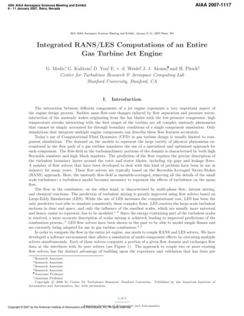
AIAA 2007-111745th AIAA Aerospace Sciences Meeting and Exhibit8 - 11 January 2007, Reno, Nevada45th AIAA Aerospace Sciences Meeting and Exhibit, January 8–11, 2007/Reno, NVIntegrated RANS/LES Computations of an EntireGas Turbine Jet EngineG. Medic , G. Kalitzin†, D. You‡, E. v. d. Weide§, J. J. Alonso¶, and H. PitschkCenter for Turbulence Research & Aerospace Computing LabStanford University, Stanford, CAI.IntroductionThe interaction between different components of a jet engine represents a very important aspect ofthe engine design process. Sudden mass flow-rate changes induced by flow separation and pressure waves,interaction of the unsteady wakes originating from the fan blades with the low-pressure compressor, hightemperature streaks interacting with the first stages of the turbine are all complex unsteady phenomenathat cannot be simply accounted for through boundary conditions of a single component simulation. Onlysimulations that integrate multiple engine components can describe these flow features accurately.Today’s use of Computational Fluid Dynamics (CFD) in gas turbine design is usually limited to component simulations. The demand on the models to represent the large variety of physical phenomena encountered in the flow path of a gas turbine mandates the use of a specialized and optimized approach foreach component. The flow-field in the turbomachinery portions of the domain is characterized by both highReynolds numbers and high Mach numbers. The prediction of the flow requires the precise description ofthe turbulent boundary layers around the rotor and stator blades, including tip gaps and leakage flows.A number of flow solvers that have been developed to deal with this kind of problem have been in use inindustry for many years. These flow solvers are typically based on the Reynolds-Averaged Navier-Stokes(RANS) approach. Here, the unsteady flow-field is ensemble-averaged, removing all the details of the smallscale turbulence; a turbulence model becomes necessary to represent the effects of turbulence on the meanflow.The flow in the combustor, on the other hand, is characterized by multi-phase flow, intense mixing,and chemical reactions. The prediction of turbulent mixing is greatly improved using flow solvers based onLarge-Eddy Simulations (LES). While the use of LES increases the computational cost, LES has been theonly predictive tool able to simulate consistently these complex flows. LES resolves the large-scale turbulentmotions in time and space, and only the influence of the smallest scales, which are usually more universaland hence, easier to represent, has to be modeled.1, 2 Since the energy-containing part of the turbulent scalesis resolved, a more accurate description of scalar mixing is achieved, leading to improved predictions of thecombustion process,.3 LES flow solvers have been shown in the past to be able to model simple flames andare currently being adapted for use in gas turbine combustors.4, 5In order to compute the flow in the entire jet engine, one needs to couple RANS and LES solvers. We havedeveloped a software environment that allows a simulation of multi-component effects by executing multiplesolvers simultaneously. Each of these solvers computes a portion of a given flow domain and exchanges flowdata at the interfaces with its peer solvers (see Figure 1). The approach to couple two or more existingflow solvers has the distinct advantage of building upon the experience and validation that has been put ResearchAssociateAssociate‡ Research Associate§ Research Associate¶ Associate Professork Assistant ProfessorCopyright c 2006 by Center for Turbulence Research, Stanford University.Aeronautics and Astronautics, Inc. with permission.† ResearchPublished by the American Institute of1 of 8AmericanInstituteAeronauticsCopyright 2007 by the American Institute of Aeronautics andAstronautics,Inc. All ofrightsreserved. and Astronautics

Figure 1. Decomposition of the engine for flow simulations.into the individual codes during their development. It provides the possibility of running simulations indifferent domains at different time steps, and provides a higher degree of flexibility. We will demonstratethis approach in a simulation of a 20o sector of the entire gas turbine jet engine, encompassing the fan, lowand high-pressure compressor, combustor, high- and low-pressure turbine, and the exit nozzle. We will showthat such a simulation can deliver important insight into the physics of interaction between different enginecomponents within a manageable turnover time, which is necessary to be useful in the design process of anengine.II.Flow solversFor the integrated computations presented here, we use flow solvers that are well-suited and tested forthe individual components: a RANS flow solver for the turbomachinery parts and an LES flow solver forthe combustor. These solvers were further adapted for efficient use on massively parallel platforms of up toseveral thousand CPUs, which are needed for these integrated computations of an entire jet engine.A.RANS flow solverThe RANS flow solver used in the computations is the SUmb code developed at the Aerospace ComputingLab (ACL) at Stanford. The flow solver computes the unsteady Reynolds-Averaged Navier-Stokes equationsusing a cell-centered discretization on arbitrary multi-block meshes.6 The solution procedure is based onefficient explicit modified Runge-Kutta methods with several convergence acceleration techniques such asmulti-grid, residual averaging, and local time-stepping. These techniques, multi-grid in particular, provideexcellent numerical convergence and fast solution turnaround. The turbulent viscosity is computed from ak ω two-equation turbulence model and adaptive wall functions are employed to compute the boundaryconditions. The dual time-stepping technique7–9 is used for time-accurate simulations that account for therelative motion of moving parts as well as other sources of flow unsteadiness.2 of 8American Institute of Aeronautics and Astronautics

B.LES flow solverThe LES flow solver used for the current study is the CDP code developed at the Center for TurbulenceResearch (CTR) at Stanford.10 Here we summarize the main features of the methodology. The filteredNavier-Stokes equations are solved in an unstructured grid system using a Smagorinsky-type subgrid-scale(SGS) model.11 The integration method used to solve the governing equations is based on a fully implicitfractional-step method. All terms, including cross-derivative diffusion terms, are advanced in time using theCrank-Nicholson method.The Cartesian components of momentum, density, and pressure are stored at the nodes of the computational elements. Once density is obtained from a flamelet library, the continuity equation can be imposed asa constraint on the momentum field, with the time-derivative of density as a source term. This constraint isenforced by the pressure, in a manner analogous to the enforcement of the incompressibility constraint forconstant density flows. The computational approach is to first advance the mixture fraction and the progressvariable. The flamelet library yields the density, whose time-derivative is then computed. The momentum ispredicted using the convective, viscous, and pressure-gradient at first. The predicted value of the momentumis then projected such that the continuity equation is satisfied.C.Boundary conditionsThe definition of the boundary conditions requires special attention, especially for LES. Because a part ofthe turbulent spectrum is resolved in the LES, the challenge is to regenerate and preserve the turbulence atthe boundaries.At the LES inflow boundary, the challenge is to prescribe transient turbulent velocity profiles fromensemble-averaged RANS data. Turbulent fluctuations at the inflow of the combustor have to be constructedusing an additional LES computation. The fluctuations can be precomputed and stored in a database,12 orcomputed on the fly from an auxililiary duct computation.13For the RANS solver, inlet and exit boundary conditions are applied using the time-averaged solutionfrom the LES.14 Turbulence variables (such as k and ω) can also be computed on the fly from a quasi-2DRANS computation of an auxilliary duct at the turbine inflow.13Figure 2. CHIMPS approach: solvers communicate location of their interface points and their mesh andsolution to the coupler. The coupler determines how to provide information to the solver at the interfacenodes.III.CHIMPS: Multi-solver couplingPrevious approaches to couple solvers were based on a pure MPI approach.15–18 In that approach, MPIis used to let different solvers communicate directly with each other. The disadvantage of this approachis that the implementation is tedious and error prone since each MPI command in one solver requires acorresponding MPI command in the other solver. Furthermore, the search and interpolation routines haveto be implemented in each solver separately.3 of 8American Institute of Aeronautics and Astronautics

A more effective approach consists in implementing all the coupling routines (communication, search,and interpolation) in a separate software module that performs these tasks: Coupler for High-PerformanceIntegrated Multi-Physics Simulations (CHIMPS).19 The solvers are now communicating with the couplersoftware only (Figure 2) and the coupler performs all searches and interpolations. In this latest version, thecoupler supports both a script language such as Python and standard programming languages like Fortran90.IV.Full-engine simulationsIn this section we present an integrated multi-component simulation of a Pratt & Whitney aircraftengine. This simulation simultaneously computes the flow in the fan/compressor, the combustor, and theturbine, and each of the components exchanges flow data with its neighbors. The goal of this simulation is todemonstrate the ability to perform complex, multi-physics, multi-code simulation on a real-world problem.The domain consists of a 20o sector of all the components; in view of the full-engine simulation, this is thesmallest sector that can be chosen since it contains one fuel injector. The initial solution for the integratedsimulation is provided by a combination of the component simulations.Note that the blade counts in turbomachinery are normally such that no sector periodicity occurs. Thisis done to avoid instabilities caused by resonance between two components. As a consequence, the trueunsteady simulation can only be done for the entire wheel, unless simplifying assumptions are made. Thecurrently accepted practice is to rescale the blade counts of the turbomachinery stages such that sectorperiodicity is obtained. To preserve the same flow blockage, the pitch of the blades is adjusted according tocommon industry practice.Figure 3. Simulation of the entire engine: axial velocity.A.Operating conditionsThe operating conditions for the engine correspond to cruise conditions; these define the boundary conditionsfor the engine: fan inlet conditions, turbine outlet conditions, and fuel inlet conditions. Boundary conditionsare also specified at the interfaces, however here they are computed using the data from the neighboringcomponent.For the fan inlet, the total temperature, total pressure, and the flow directions are imposed. At theoutlet of the compressor, the static pressure is imposed. The combustor receives at the inlet the flow vector[u, v, w]. The fuel mass flow rate is defined corresponding to the cruise operating conditions. The actualoutlet of the combustor domain is far downstream in order to minimize the effect of the domain boundary4 of 8American Institute of Aeronautics and Astronautics