Transcription
Journal of Applied Fluid Mechanics, Vol. 12, No. 6, pp. 1801-1812, 2019.Available online at www.jafmonline.net, ISSN 1735-3572, EISSN 1735-3645.DOI: 10.29252/jafm.12.06.29538Comparison of Interface Description Methods Availablein Commercial CFD SoftwareA. A. Barral Jr.1, R. B. Minussi2 and M. V. Canhoto Alves1†Department of Petroleum Engineering – Santa Catarina State University, Balneário Camboriú, SantaCatarina, 88.336-275, Brazil2Centre of Marine Studies – Federal University of Paraná, Pontal do Paraná, Paraná, 83.255-976, Brazil1†Corresponding Author e-mail: marcus.alves@udesc.br(Received August 16, 2018; accepted January 22, 2019)ABSTRACTThis study addresses the characteristics of the interpolation functions and interface reconstructionroutines for the VOF – Volume of Fluid method available in the commercial CFD software ANSYSFLUENT. This software was used because it has both implicit and explicit VOF approaches along withdiverse interpolation functions. Some of these functions were compared from different viewpoints: thequality of the reconstructed interface; the ability to preserve the initial mass inside the system (numericaldiffusion); and the computing time. To undertake the qualitative and quantitative comparisons, a testproblem that combines the classical dam break and slosh tank benchmark problems was used. Noanalytical solution available was found for this problem, in which the most interesting feature is a highinteraction between the velocity field and volume fraction, thus making it ideal for addressing the issueof interface smearing. ANSYS-FLUENT permits using 5 interpolation functions for transientsimulations: PLIC, CICSAM, HRIC (explicit and implicit) and the UPWIND scheme, and four whenperforming steady state ones: BGM, modified HRIC, COMPRESSIVE and UPWIND schemes. Bothtransient and steady state solutions were analyzed in this study, using all the above schemes, except theUPWIND one for steady state simulations. It was found that, for thinner grids, PLIC, CISAM and theexplicit HRIC schemes had similar performances concerning the quality of the reconstructed interfaceand mass conservation. On the other hand, PLIC shows the best results for coarser grids, being the onlyto conserve mass for all tests. The computation time was similar for all transient simulation (within eachgrid). Concerning the steady state simulations, which are, in fact, distorted transient simulations, theBGM and the COMPRESSIVE schemes produced similar results, but BGM consumed morecomputational time.Keywords: Volume of Fluid; Numerical Diffusion; Interfacial Smearing.NOMENCLATUREqStu vrate of shear tensormass transfer flux between phasespth phase (when in a subscript)Thermodynamic pressureqth phasemass source termtimevelocity componentvelocity dynamic viscosityVxvelocity moduluscoordinate system componentṁpα S μρ Re Eo 1VL 1 1VL ReCa Eovolume fractionDirac’s delta function at the interfaceinterface mean curvaturedynamic viscosityspecific masssurface tensionReynolds numberEötvös numberCapillary Number
A. A. Barral Jr. et al. / JAFM, Vol. 12, No. 6, pp. 1801-1812, 2019.1.Calculation). The basic difference is that CLSVOFand PLIC use geometric interface reconstruction,different from methods THINC/SW and WLIC,which does not require such geometricreconstruction, i. e., does not need to calculate theslope of the interface, using only weightedfunctions (WLIC) or a tangent fitted curve(THINC/SW). All methods are implemented usingFORTRAN, and the comparison was done bymeasuring mass conservation, spurious currents,parasitic currents, CPU time and number of codelines. Aniszewski et al. (2014) point out that allmethods have their own advantages anddisadvantages. As methods THINC/SW and WLICare simpler, they require much less computationallines and then their use would be preferable in thefirst attempts for a programmer to study a twophase flow. Furthermore, using THINC/SW orWLIC VOF methods coupled with Level Setretrieves much more accurate results concerning themass conservation then using Level Set alone.When simulating surface tension dominated flowsor highly fragmented interface flows, CLSVOF andPLIC can be less expensive than using THINC/SWand WLIC, as the latter requires refined grids.Overall, the differences between THINC/SW andWLIC and between CLSVOF and PLIC are muchsmaller then between CLSVOF or PLIC andTHINC/SW or WLIC.INTRODUCTIONThe VOF method can model the flow of two ormore fluids by solving a single set of momentumequations and tracking the volume fraction ofeach of the fluid phase throughout the domain.Typical applications of the VOF model are forimmiscible fluid flow and include the predictionof jet breakup, the motion of large bubbles in aliquid, the motion of liquid after a dam break, andthe steady or transient tracking of any interphaseinterface.For each additional phase to model, a variable mustbe introduced: the volume fraction of the phase ineach computational cell. In each control volume, thesum of volume fractions of all phases must be equalto one. The fields for all variables and properties areshared by the phases and represent volumeaveraged values (if the volume fraction of each ofthe phases is known at each location and time).Thus, the variables and properties in any given cellare either purely representative of one of the phases,or representative of a mixture of the phases,depending upon the volume fraction values. Basedon the local volume fraction, the appropriateproperties and variables are assigned to each controlvolume within the domain.The VOF model has been used in the literature tosimulate several complex problems in engineering,such as: the transient behavior of lubricant insidehermetic compressors (Lückmann et al., 2009; andAlves et al. 2011 & 2013); two phase flows in tubesand ducts (Soleymani et al., 2008; Da Riva and DelCol, 2009; Kashid et al., 2010; Hernandez-Perez etal., 2011; Horgue et al., 2012; Magnini et al., 2013;Ratkovich et al., 2013; Karami et al., 2014; Saad etal., 2014; Bortolin et al., 2014); modeling of theRayleigh-Taylor Instabilities (Bilger et al. 2017);simulation of the dam break problem (Minussi andMaciel, 2012; Caron et al., 2015). Although veryuseful, the VOF model has limitations speciallyregarding the momentum transfer through theinterface (Rezende et al., 2014). Rezende et al.(2014) developed a novel approach to close theinterfacial modeling for two-phase flow modelingwith the VOF method.Caron et al. (2014) show a comparison of the dambreak problem between experimental data andnumerical simulations using the VOF model. Thecomparison is focused on the turbulence modelsavailable, comparing the results with theexperimental results. The results show theturbulence models introduce a diffusive effect thathelps in the control of the interface evolution. Thiseffect allows obtaining a mesh independent solutionwith less volumes.Cifani et al. (2016) compare two VOF advectionmethods using openFOAM, a high order differentialscheme (the surface compression method) and thePLIC (implemented as a user-defined function). Therising air bubble inside a viscous fluid test problemwas considered, and the authors concluded that,although the compression method always conservesmass and is less computationally expensive, itsresults are not as accurate. The authors speculatethat the main reason is interface numerical diffusionproblems. The PLIC shows a 2nd orderconvergence rate in most of the test cases, highaccuracy in describing the interface and a verysmall mass imbalance. Cifani et al. (2016) alsopoint out that the combination of the VOF-PLICwith a surface tension computation using asmoothing technique shows the best results (both inaccuracy and grid refinement convergenceanalysis).The open literature also has several studies dealingwith the comparison of several interface descriptionmethods. These comparisons deal mainly withcodes developed in house and implemented using acompiler of choice. Most notably the studies rangefrom the pioneer comparisons of Scardovelli andZaleski (1999) and Pilliod and Puckett (2004) tomore recent studies by: Klostermann et al. (2012);Aniszewski et al. (2014); Caron et al. (2014);Cifani et al. (2016).Aniszewski et al. (2014) compare 4 types ofadvection methods in the CLSVOF (Coupled LevelSet Volume of Fluid) framework. The algorithmscompared are: the CLSVOF; the THINC/SWmethod (Tangent of Hyperbola Interface Capturingwith Slope Weighting); the WLIC method(Weighted Linear Interface Calculation); and, thePLIC method (Piece-wise Linear Interface2.MODELINGThe tracking of the interface between the phases isaccomplished by solving a continuity equation forthe volume fraction of each of the phases. For the1802
A. A. Barral Jr. et al. / JAFM, Vol. 12, No. 6, pp. 1801-1812, 2019. v p v v 2 D 2 S nˆ t q th phase, this equation has the following form: q q t v Sqq q qn m pq m qp (1)in which D is the rate of shear tensor, and the lastterm of Eq. (5), 2 S nˆ , is due to the surfacetension force acting on the interface. The mostcommon surface tension model used in literature isthe Continuum Surface Force – CSF modelproposed by Brackbill et al. (1992) and is theprocedure adopted in this study. With this model,the addition of surface tension to the VOFcalculation results in a source term in themomentum equation (last term in Eq. 5).p 1In which: q is the q th phase volume fraction,m pq is the mass transfer from phase p to phaseand m qp is the mass transfer from phase q to phasep . The source term on the right-hand side of Eq.(1), S q is usually zero, but it can be specified to bea mass generation term due to any chemicalreaction in the bulk of each phase.The only properties that are not continuous throughthe interface are density and viscosity. These arecalculatedrespectively by thefollowingexpressions,After properly solving the transport equations andvolume fraction equations, the algorithm of theVOF model must reconstruct the interface betweenthe phases and propagate such interface. These twosteps are so important in the VOF model thatusually the VOF method is said to be divided in twosteps: reconstruction of the interface, and advectionof the interface (Parker and Youngs, 1992; Riderand Kothe; 1998; Scardovelli and Zaleski, 1999;Pilliod and Puckett, 2004). Specific algorithmsperform each of these steps, and special attention isgiven to the reconstruction, because this stepdictates the resolution of the interface. For theadvection there are two algorithms, the operatorsplit and the unsplit, as explained by Scardovelliand Zaleski (1999) to be respectively, explicit andimplicit temporal algorithms. q q (7)nq 1As previously said, the application of the VOFmethod is divided in two steps: ruction. The first step of the VOF methodis the advection of the interface (or the volumefractions), it is meant to determine how theinterface will evolve between two consecutivetime steps. The second step is to reconstruct theinterface, and it is meant to determine the shape,orientation and current position of the interface atthe end of any given time step. This is performedusing the solution of the motion equations (massand momentum conservation equations) alongwith the volume fraction advection equation (Eq.3).The advection of the interface is determined bysolving the motion equations based on the shape,orientation and the position of the interface at thebeginning of any given time step. This process mustavoid the interface smearing, so the numericalsolution must guarantee low levels of numericaldiffusion. According to the ANSYS-FLUENT SolverTheory Guide (2017), three basic methods foradvection can be found in literature: the originaldonor-acceptor scheme (algorithm splitting)presented by Hirt and Nichols (1981), whichcomputes the face fluxes in each directionseparately; the high-order differencing schemessuch as the CICSAM (Compressive InterfaceCapturing Scheme for Arbitrary Meshes) presentedby Ubbink (1997), or the unsplit algorithm thatcomputes the face fluxes in all directions at once;and the line techniques, which are, in essence,improvements in the donor-acceptor scheme. Theline techniques differ from the donor-acceptorscheme in the fact that the fluxes for each phase areweighted depending on the inclination of the line(or plane in 3D) that separates the phases insideeach cell (ANSYS-FLUENT Solver Theory Guide,2017). Each of these employs its ownThe motion of the interface is described by thevolume fraction equation (Eq. (1) with no sourceterm, no mass transfer and for an incompressibleflow) and may be written as, t(6)q 1The conservation of mass in an interface with nophase change or mass transfer establishes that: (2)vq nˆ V vq q 0 q q nAn interfacial surface can be geometricallyrepresented in several ways (Whitman, 1974). In theVOF method, the interface itself is not tracked,instead, the procedure consists of evolving thematerial volume through each computational cell intime and reconstructing the interface. Thereconstruction is based on solving the motionequations, comprising the conservation equations ofmass and momentum for transient, incompressibleflow of Newtonian fluids. q(5)(3)The software adopted, ANSYS-FLUENT (ANSYSFLUENT Solver Theory Guide, 2017; ANSYSFLUENT User Guide, 2017), uses a whole domainformulation for solving equations of motion (inother words, it solves only one set of motionequations for the role domain). The form of theequations of motion appears below, respectivelymass and momentum conservation equations, v 0(4)1803
A. A. Barral Jr. et al. / JAFM, Vol. 12, No. 6, pp. 1801-1812, 2019.reconstruction technique.approach is displayed as small dots. Although thegrid used is the same (3.125 mm regular spacing),the results of Klostermann et al. (2013) are shownas few points due to the lack of the original data forcomparison. These points were captured with an inhouse code that allows for the capturing of discretepoints in digital images.The ANSYS-FLUENT software offers twointegration procedures for Eq. (3), implicit(available for transient and steady state simulations)and explicit (for transient simulations only). Thegreat advantage of the implicit integration is that,when only the steady state solution is desired, theuse of the implicit integration process can be muchmore computationally efficient and less timedemanding, while the explicit integration demandsfor the solution of the full transient flow. Theimplicit integration can also be used for establishinginitial conditions for transient simulations, speedingup the process.Table 1 Physical properties and dimensionlessparameters for the rising bubble simulationsCase TC1Case TC2The methodologies to be compared in this studyare the following: Geometric Reconstruction(based on the PLIC – Piecewise Linear InterfaceConstruction), which is a line technique; theCICSAM, the HRIC – High Resolution InterfaceCapturing, the Compressive Scheme, the BoundedGradient Maximization Scheme – BGM, are highorder differencing schemes; and the UPWINDInterpolation Scheme based on the donor-acceptorscheme. The use of the Geometric Reconstructionand the CICSAM algorithms are limited totransient simulations because these are based onthe explicit solution for the interface (operatorsplitting method). The HRIC and the UPWINDschemes can be used within both transient andsteady state simulations, using the splittingoperator for the transient calculations and animplicit unsplit operator scheme for steady state.The BGM scheme can only be used for steadystate simulations. These methodologies areextensively described in several texts in literature(Parker and Youngs, 1992; Ubbink, 1997; Riderand Kothe; 1998; Scardovelli and Zaleski, 1999;Muzaferiju and Peric, 2000; Pilliod and Puckett,2004; Walters and Wolgemuth, 2009) and will notbe extensively discussed Eo10125Ca0.2863.571(a)SOLUTION VALIDATIONTo validate the numerical solutions obtained usingANSYS-FLUENT, the single rising bubble in aviscous liquid was chosen as benchmark. TheGeometric Reconstruction algorithm was used forboth simulated cases, because this method will beused for creating the reference solution of the dambreak problem. The study by Klostermann et al.(2013) is used for comparisons. This study wascompared with other numerical simulations (forinterface form and bubble rise velocity) and withexperimental data (for bubble rise velocity). Thenumerical parameters for the simulations were thesame as in the original study, with a regular gridspacing of 3.125 mm and 1.5625 ms as timeinterval. The conditions, physical properties anddimensionless numbers for the simulations areshown in Table 1.(b)Fig. 1. Comparison with the study byKlostermann et al. (2013) at 1.5 s (a) and 3.0 s (b)for the TC1 case.Figure 2 shows a comparison analogous to that ofFig. 1, with the conditions, physical propertiesand dimensionless numbers for case TC2. Thefigure shows the current results as small dots andthe reference simulation (Klostermann et al.,2013) as triangles. The simulation using theFigure 1 shows the comparison of interface form forcase TC1. The comparison shows the two solutionsare almost coincident. The results of Klostermann etal. (2013) are shown in triangles and the current1804
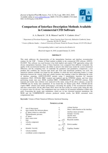
A. A. Barral Jr. et al. / JAFM, Vol. 12, No. 6, pp. 1801-1812, 2019.ANSYS-FLUENT (current approach) was able toreproduce the results of Klostermann et al.(2013), including the bubble break-up at theedges and the trailing small bubbles in each tip ofthe main bubble.Table 2 Naming of computational grids used forsimulation and comparisonThousands ofGrid Number Grid Division ComputationalCells1100 x 2022200 x 4083400 x 80324800 x 160128With this results, the solutions for the dam breakproblem can now be addressed with confidence, andthe ANSYS-FLUENT software will be able to dealwith the interfacial break-up and reconnection,while still being able to correctly represent theinterface evolution.A single geometric reconstruction (PLIC)simulation with 512 thousand volumes (1600 x 320computational cells) was executed and is taken asthe benchmark for comparison with all othersimulations. In this benchmark simulation, the timestep was also reduced to 0.1 ms, while also allowingfor 100 interactions within each time step. Thedefault settings for solution methods and underrelaxation parameters were maintained. Figure 4shows a grid refinement assessment for all thesimulated grids using the geometric reconstruction(PLIC) and demonstrates that the simulation withgrid 4 and the reference grid of 512 thousandvolumes present the same results. Figure 5 showsthe reference simulation in several time steps (from0.5 s to 1.9 s).After starting the simulation, water runs through thebase wall and reaches the right wall (sloshing) nearthe 0.5 s mark. At the 0.7 s, the water front fallsback to the bottom wall. After the impact betweenthe water front and the liquid film at the bottomwall, the mixing phenomenon is apparent. The airbubbles became entrapped into water, revealing ahighly nonlinear interaction between the phaseadvection and the velocity field. This entrance of airinside the water phase continues until the phaseseparation starts to become prominent near thesteady state. As one of the focuses of this study is toinvestigate the quality of the interfacialrepresentation, the result analysis will beconcentrated between the instants 1.0 s and 1.3 s.(a)For the steady state simulations, all defaultparameters were maintained; however, the steadystate calculations performed by ANSYS-FLUENTsoftware are in fact pseudo-transient simulations,with a distorted time advancement. The procedureis to advance time while not fully converging eachtime interval. A time scale is provided to thesoftware along with a Courant number and amaximum simu
in Commercial CFD Software. . comparison is focused on the turbulence models available, comparing the results with the experimental results. The results show the turbulence models introduce a diffusive effect that helps in the control of