Transcription
2.29 Numerical Fluid MechanicsSpring 2015 – Lecture 19REVIEW Lecture 18: Solution of the Navier-Stokes Equations v .( v v ) p 2v g t0 .v – Discretization of the convective and viscous terms– Discretization of the pressure term– Conservation principles22 up p g.r .u ( p ei gi xi ei j ei )33 x j S p ei .ndS Momentum and Mass Energy22vv dV (v .n )dA p v .n dA ( .v ). n dA : v p .v g.v dV CSCSCSCV22 t CV – Choice of Variable Arrangement on the Grid Collocated and Staggered– Calculation of the Pressure . p 2 p .2.29 v . .( v v ) . 2v . g . .( v v ) tNumerical Fluid Mechanics p ui u j xi xi xi x j PFJL Lecture 19,1
2.29 Numerical Fluid MechanicsSpring 2015 – Lecture 19REVIEW Lecture 18, Cont’d: Solution of the Navier-Stokes Equations– Pressure Correction Methods: i) Solve momentum for a known pressure leading to new velocity, thenii) Solve Poisson to obtain a corrected pressure andiii) Correct velocity (and possibly pressure), go to i) for next time-step. A Forward-Euler Explicit (Poisson for p at tn, then mom. for velocity at tn 1) A Backward-Euler Implicit ui n 1 ui n ( ui u j ) n 1 ij n 1 p n 1 t x x xi jj p n 1 ( ui u j ) xi xi xi xjn 1 ij n 1 x j – Nonlinear solvers, Linearized solvers and ADI solvers Steady state solvers, implicit pressure correction schemes: iterate using– Outer iterations:uim*A um*i bm 1uim*δp δxi– Inner iterations:2.29m 1uim*uimmibut require A u bmiA ubmuim*δp δximuimmδpδ uimδ uim* δ uim* and 0 0 Aδxiδxiδxiδxi 1mδp δxi mNumerical Fluid MechanicsPFJL Lecture 19,2
2.29 Numerical Fluid MechanicsSpring 2015 – Lecture 19REVIEW Lecture 18, Cont’d: Solution of the Navier-Stokes Equations– Projection Correction Methods:– Construct predictor velocity field that does not satisfy continuity, then correct itusing a pressure gradient– Divergence producing part of the predictor velocity is “projected out” Non-Incremental:– No pressure term used in predictor momentum eq. Incremental:– Old pressure term used in predictor momentum eq. Rotational Incremental:– Old pressure term used in predictor momentum eq.– Pressure update has a rotational correction: p2.29Numerical Fluid Mechanicsn 1 p n p ' p n p n 1 f (u ')PFJL Lecture 19,3
TODAY (Lecture 19) Solution of the Navier-Stokes Equations– Pressure Correction Methods Projection Methods– Non-Incremental, Incremental and Rotational-incremental Schemes– Fractional Step Methods: Example using Crank-Nicholson– Streamfunction-Vorticity Methods: scheme and boundary conditions– Artificial Compressibility Methods: scheme definitions and example– Boundary Conditions: Wall/Symmetry and Open boundary conditions Time-Time-Marching Methods and ODEs. – Initial Value Problems– Euler’s method– Taylor Series Methods Error analysis– Simple 2nd order methods Heun’s Predictor-Corrector and Midpoint Method (belong to Runge-Kutta’smethods)2.29Numerical Fluid MechanicsPFJL Lecture 19,4
References and Reading Assignments Chapter 7 on “Incompressible Navier-Stokes equations” of“J. H. Ferziger and M. Peric, Computational Methods forFluid Dynamics. Springer, NY, 3rd edition, 2002” Chapter 11 on “Incompressible Navier-Stokes Equations” ofT. Cebeci, J. P. Shao, F. Kafyeke and E. Laurendeau,Computational Fluid Dynamics for Engineers. Springer,2005. Chapter 17 on “Incompressible Viscous Flows” of Fletcher,Computational Techniques for Fluid Dynamics. Springer,2003.2.29Numerical Fluid MechanicsPFJL Lecture 19,5
Projection Methods: Example Scheme 3Guermond et al, CM-AME-2006Rotational Incremental (Timmermans et al, 1996): Old pressure term used in predictor momentum equation Correct pressure based on continuity: p n 1 p n p ' p n p n 1 f (u ') Update velocity using pressure increment in momentum equation u i* n 1 ui n 1 ui uin ( ui u j ) n 1 ij n 1 p n t ; xxxjji * n 1 ui xi ui n 1 ui t xin 1* n 1 0 tp n 1 p n p n 1 2.29 p n 1 p n 1 xi xi ui* n 1 u i* n 1n 1 p 1 t xi xi xi D (bc) u ;i* n 1 ui u j x xi j ij n 1 p n 1 n 0 DNotes:- this scheme accounts for u’ in the pressure eqn.- It can be made into a SIMPLE-like method, if iterations are added- Again, the advection term can be explicit or implicit. The rotationalcorrection to the left assumes explicit advectionNumerical Fluid MechanicsPFJL Lecture 19,6
Other Methods: Fractional Step Methods In the previous methods, pressure is used to:– Enforce continuity: it is more a mathematical variable than a physical one– Fill the RHS of the momentum eqns. explicitly (predictor step for velocity) The fractional step methods (Kim and Moin, 1985) generalize ADI– But works on term-by-term (instead of dimension-by-dimension). Hence,does not necessarily use pressure in the predictor step– Let’s write the NS equations a in symbolic form:uin 1 uin (Ci Di Pi ) twhere Ci, Di and Pi represent the convective, diffusive and pressure terms– The equation is readily split into a three-steps method:ui* uin Ci tui** ui* Di tuin 1 ui** Pi t– In the 3rd step, the pressure gradient ensures uin 1 satisfy the continuity eq.2.29Numerical Fluid MechanicsPFJL Lecture 19,7
Fractional Step Methods, Cont’d Many variations of Fractional step methods exists– Pressure can be a pseudo-pressure (depends on the specific steps, i.e.what is in ui** , Pi )– Terms can be split further (one coordinate at a time, etc.)– For the time-marching, Runge-Kutta explicit, direct 2nd order implicit orCrank-Nicholson scheme are often used– Linearization and ADI are also used– Used by Choi and Moin (1994) with central difference in space for directsimulations of turbulence (Direct Navier Stokes, DNS) Next, we describe a scheme similar to that of Choi and Moin,but using Crank-Nicholson2.29Numerical Fluid MechanicsPFJL Lecture 19,8
Fractional Step Methods:Example based on Crank-Nicholson In the first step, velocity is advanced using: ui * ui n t H (ui ) H (ui ) pn – Pressure from the previous time-step*2n xi – Convective, viscous and body forces are represented as an average of old andnew values (Crank-Nicolson)– Nonlinear equations iterate, e.g. Newton’s scheme used by Choi et al (1994) Second-step: Half the pressure gradient term is removed from ui*, to lead ui** ui ** ui * 1 pn t 2 xi Final step: use half of the gradient of the still unknown new pressure ui n 1 ui ** 1 p n 1 t 2 xi New velocity must satisfy the continuity equation (is divergence free):– Taking the divergence of final step: p n 1 2 ( ui )** xi xi t xi– Once pn 1 is solved for, the final step above gives the new velocities2.29Numerical Fluid MechanicsPFJL Lecture 19,9
Fractional Step Methods:Example based on Crank-Nicholson Putting all steps together: ui n 1 ui n H (uin ) H (ui* ) 1 p n p n 1 t 22xx i i – To represent Crank-Nicolson correctly, H(ui* ) should be H(uin 1 )– However, we can show that the splitting error, uin 1 - ui* , is 2nd order in time andthus consistent with C-N’s truncation error: indeed, subtract the first step from then 1complete scheme, to obtain, t p pn t 2 p n 1* ui – With this, one also obtains: ui ui n 1 ui * 2 xi xi 2 xi t t ( p n 1 p n ) t ( p ' ) 22 xi xiwhich is similar to the final step, but has the form of a pressure-correction on ui* .This later eq. can be used to obtain a Poisson eq. for p’ and replace that for pn 1 Fractional steps methods have become rather popular– Many variations, but all are based on the same principles (illustrated by C-N here)– Main difference with SIMPLE-type time-marching schemes: SIMPLE schemessolve the nonlinear pressure and momentum equations several times per timestep in outer iterations (iterative nonlinear solve)2.29Numerical Fluid MechanicsPFJL Lecture 19,10
Incompressible Fluid(review Lecture 8-NS)Vorticity EquationVorticityNavier-Stokes Equationcurl of Navier-Stokes Equation2.29Numerical Fluid MechanicsPFJL Lecture 19,11
Streamfunction-Vorticity Methods For incompressible, 2D flows with constant fluid properties, NScan be simplified by introducing the streamfunction ψ andvorticity ω as dependent variablesu , v y xand v u x y(ω v )– Streamlines (lines tangent to velocity): constant ψ– Vorticity vector is orthogonal to plane of the 2D flow u v 0 ! x y v uleadsu and v in y x x y– 2D continuity is automatically satisfied: In 2D, substitutingkinematic condition:to the 2 2 2 2 x y The vertical component of the vorticity dynamical equationleads: 2 2 2.29 t u x v y 2 2 y xNumerical Fluid MechanicsPFJL Lecture 19,12
Streamfunction-Vorticity Methods, Cont’d Main advantages:– Pressure does not appear in either of these equations!– 2D-NS has been replaced by a set of 2 coupled PDEs Instead of 2 velocities and 1 pressure, we have only two dependent variables Explicit solution scheme– Given initial velocity field, compute vorticity by differentiation– Use this vorticity ωn in the RHS of the dynamical equation for vorticity, toobtain ωn 1– With ωn 1 the streamfunction ψn 1 can be obtained from the Poissonequation With ψn 1, we can differentiate to obtain the velocity– Continue to time n 2, and so on One issue with this scheme: boundary conditions2.29Numerical Fluid MechanicsPFJL Lecture 19,13
Streamfunction-Vorticity Methods, Cont’dBoundary conditions Boundary conditions for ψ– Solid boundaries are streamlines and require: ψ constant– However, values of ψ at these boundaries can be computed only ifvelocity field is known Boundary conditions for ω– Neither vorticity nor its derivatives at the boundaries are known inadvance u– For example, at the wall: “ wall wall / ” since wall ywall Vorticity at the wall is proportional to the shear stress, but the shear stress isoften what one is trying to compute 2 2 2 ,– Boundary values for ω can be obtained from2 x y 2 i.e. one-sided differences at the wall: 2 nbut this usually converges slowly and can require refinement– Discontinuities also occur at corners2.29Numerical Fluid MechanicsPFJL Lecture 19,14
Streamfunction-Vorticity Methods, Cont’d– Discontinuities also occur at corners for vorticity The derivatives v uand x yare not continuous at A and B This means special treatment for v u x yABCDImage by MIT OpenCourseWare.e.g. refine the grid at corners Vorticiy-streamfunction approach useful in 2D, but is now lesspopular because extension to 3D difficult– In 3D, vorticity has 3 components, hence problem becomes as/moreexpensive as NS– Streamfunctiom is still used in quasi-2D problems for example, in the ocean or in the atmosphere, but even there, it has beenreplaced by level-based models with a free-surface (no steady 2D continuity)2.29Numerical Fluid MechanicsPFJL Lecture 19,15
Artificial Compressibility Methods Compressible flow is of great importance (e.g. aerodynamicsand turbine engine design) Many methods have been developed (e.g. MacCormack,Beam-Warming, etc) Can they be used for incompressible flows? Main difference between incompressible and compressible NSis the mathematical character of the equations– Incompressible eqs.: no time derivative in the continuity eqn: .v 0 They have a mixed parabolic-elliptic character in time-space– Compressible eqs.: there is a time-derivative in the continuity equation: They have a direct hyperbolic character: Allow pressure/sound waves .( v ) 0 t– How to use methods for compressible flows in incompressible flows?2.29Numerical Fluid MechanicsPFJL Lecture 19,16
Artificial Compressibility Methods, Cont’d Most straightforward: Append a time derivative to the continuity equation– Since density is constant, adding a time-rate-of-change for ρ not possible– Use pressure instead (linked to ρ via an eqn. of state in the general case):1 p ui 0 t xi where β is an artificial compressibility parameter (dimension of velocity2) Its value is key to the performance of such methods:– The larger/smaller β is, the more/less incompressible the scheme is– Large β makes the equation stiff (not well conditioned for time-integration) p Methods most useful for solving steady flow problem (at convergence: 0) tor inner-iterations in dual-time schemes.– To solve this new problem, many methods can be used, especially Time-marching schemes: what we have seen & will see (R-K, multi-steps, etc) Finite differences or finite volumes in space Alternating direction method is attractive: one spatial direction at a time2.29Numerical Fluid MechanicsPFJL Lecture 19,17
Artificial Compressibility Methods, Cont’d Connecting these methods with the previous ones:– Consider the intermediate velocity field (ρui* )n 1 obtained from solvingmomentum with the old pressure– It does not satisfy the incompressible continuity equation: There remains an erroneous time rate of change of mass flux ( ui * )n 1 * xi t method needs to correct for it Example of an artificial compressibility scheme– Instead of explicit in time, let’s use implicit Euler (larger time steps forn 1stiff term with large β)p n 1 p n ( ui ) t xi 0– Issue: velocity field at n 1 not known coupled ui and p system solve– To decouple the system, one could linearize about the old(intermediate) state and transform the above equation into a Poissonequation for the pressure or pressure correction!2.29Numerical Fluid MechanicsPFJL Lecture 19,18
Artificial Compressibility Methods:Example Scheme, Cont’d Idea 1: expand unknown ui using Taylor series in pressure ( u ) derivatives(p p )(p p ) u u n 1ii* n 1 p in 1* n 1n*n 1n– Inserting (ρui )n 1 in the continuity equation leads an equation for pn 1 n 1* n 1 p n 1 p n ( u)*n 1ni ui ( p p ) 0 t xi p n 1 p n 1 ( ui * ) – Expressing in terms of x using N-S, this is a Poisson-like pn 1i pn 1- pn ! ( ui * ) p n 1 p nn 1* n 1 ( ) ui ui Idea 2: utilize directly p xi xi xi eq. for– Then, still take divergence of (ρui* )n 1 and derive Poisson-like equation Ideal value of β is problem dependent– The larger the β, the more incompressible. Lowest values of β can be computed byrequiring that pressure waves propagate much faster than the flow velocity orvorticity speeds2.29Numerical Fluid MechanicsPFJL Lecture 19,19
Numerical Boundary Conditions for N-S eqns.:Velocity At a wall, the no-slip boundary condition applies:– Velocity at the wall is the wall velocity (Dirichlet)– In some cases (e.g. fully-developed flow), the tangential velocity is constantalong the wall. By continuity, this implies no normal viscous stress: u 0 x wall yy 2 v y v yyy 0nWwallυuPweEυsuS 0Near-boundary CVWallwallSymmetry planeOn the boundary conditions at a wall and a symmetry planeImage by MIT OpenCourseWare.– For the shear stress:FSshear xy dS SSSS uu uSdS S SS P yyP yS At a symmetry plane, it is the opposite:– Shear stress is null: xy – Normal stress is non-zero: yy 2 2.29 u 0 FSshear 0 y symv v v vdS 2 S S S P S 0 FSnormal yy dS 2 SSSSyP yS y sym yNumerical Fluid MechanicsPFJL Lecture 19,20
Numerical Boundary Conditions for N-S eqns.:Pressure Wall/Symmetry Pressure BCs for the Momentum equations– For the momentum equations with staggered grids, the pressure is notrequired at boundaries (pressure is computed in the interior in the middleof the CV or FD cell)– With collocated arrangements, values at the boundary for p are needed.They can be extrapolated from the interior (may require grid refinement) Wall/Symmetry Pressure BCs for the Poisson equation– When the mass flux (velocity) is specified at a boundary, this means that: Correction to the mass flux (velocity) at the boundary is also zero This affects the continuity eq., hence the p eq.: zero normal-velocity-correction often means gradient of the pressure-correction at the boundary is then alsozeroyy(take the dot product of thevelocity correction equationwith the normal at the bnd)nWυuPweEυsuSWallNear-boundary CVSymmetry planeOn the boundary conditions at a wall and a symmetry planeImage by MIT OpenCourseWare.2.29Numerical Fluid MechanicsPFJL Lecture 19,21
Numerical BCs for N-S eqns:Outflow/Outlet Conditions Outlet often most problematic since information is advected from the interiorto the (open) boundary If velocity is extrapolated to the far-away boundary, u 0 e.g., uE uP , n– It may need to be corrected so as to ensure that the mass flux is conserved(same as the flux at the inlet)– These corrected BC velocities are then kept fixed for the next iteration. Thisimplies no corrections to the mass flux BC, thus a von Neumann condition for thepressure correction (note that p itself is linear along the flow if fully developed).– The new interior velocity is then extrapolated to the boundary, etc.– To avoid singularities for p (von Neumann at all boundaries for p), one needs tospecify p at a one point to be fixed (or impose a fixed mean p) If flow is not fully developed: u 0 n p ' 0 n e.g. 2u 0 or n 2 2 p ' 0 n 2 If the pressure difference between the inlet and outlet is specified, then thevelocities at these boundaries can not be specified.– They have to be computed so that the pressure loss is the specified value– Can be done again by extrapolation of the boundary velocities from the interior:these extrapolated velocities can be corrected to keep a constant mass flux. Much research in OBC in ocean modeling2.29Numerical Fluid MechanicsPFJL Lecture 19,22
MIT OpenCourseWarehttp://ocw.mit.edu2.29 Numerical Fluid MechanicsSpring 2015For information about citing these materials or our Terms of Use, visit: http://ocw.mit.edu/terms.
2.29 Numerical Fluid Mechanics Spring 2015 -L. 2.29 Numerical Fluid Mechanics PFJL Lecture 19, 2. ecture 19. REVIEW Lecture . 18, Cont'd: Solution of the Navier-Stokes Equations -Pressure Correction Methods: i) Solve momentum for a known pressure leading to new velocity, then ii) Solve Poisson to obtain a corrected pressure and