WIXLIB

Chapter 0PrefaceThis is a book about statistical mechanics at the advanced undergraduate level. It assumes a background inclassical mechanics through the concept of phase space, in quantum mechanics through the Pauli exclusionprinciple, and in mathematics through multivariate calculus. (Section 9.2 also assumes that you can candiagonalize a 2 2 matrix.)The book is in draft form and I would appreciate your comments and suggestions for improvement. Inparticular, if you have an idea for a new problem, or for a new class of problems, I would appreciate hearingabout it. If you are studying statistical mechanics and find that you are asking yourself “Why is. . . true” or“What would happen if. . . were changed?” or “I wish I were more familiar with. . . ”, then you have the germof a new problem. . . so please tell me!The specific goals of this treatment include: To demonstrate the extraordinary range of applicability of the ideas of statistical mechanics. Theseideas are applicable to crystals and magnets, superconductors and solutions, surfaces and even bottlesof light. I am always irritated by books that apply statistical mechanics only to fluids, or worse, onlyto the ideal gas. To introduce some modern concepts and tools such as correlation functions and computer simulation.While a full treatment awaits the final two chapters, the need for these tools is presented throughoutthe book. To develop qualitative insight as well as analytic and technical skills. Serving this goal are particularsections of text (e.g. section 2.6) and particular problems (e.g. problem 2.4) as well as overall attentionto conceptual issues. Also in support of this goal is an attempt to eliminate misconceptions as wellas present correct ideas (see appendix I, “Catalog of Misconceptions”). I particularly aim to foster aqualitative understanding of those central concepts, entropy and chemical potential, emphasizing thatthe latter is no more difficult to understand (and no less!) than temperature.1

2CHAPTER 0. PREFACE To review classical and quantum mechanics, and mathematics, with a special emphasis on difficultpoints. It is my experience that some topics are so subtle that they are never learned on first exposure,no matter how well they are taught. A good example is the interchange rule for identical particlesin quantum mechanics. The rule is so simple and easy to state, yet its consequences are so dramaticand far reaching, that any student will profit from seeing it treated independently in both a quantummechanics course and a statistical mechanics course. To develop problem solving skills. In the sample problems I attempt to teach both strategy andtactics—rather than just show how to solve a problem I point out why the steps I use are profitable.(See the index entry on “problem solving tips”.) Throughout I emphasize that doing a problem involvesmore than simply reaching an algebraic result: it also involves trying to understand that result andappreciate its significance.The problems are a central part of this book. (Indeed, I wrote the problems first and designed the bookaround them.) In any physics course, the problems play a number of roles: they check to make sure youunderstand the material, they force you to be an active (and thus more effective) participant in your ownlearning, they expose you to new topics and applications. For this reason, the problems spread over a widerange of difficulty, and I have identified them as such. Easy problems (marked with an E) might better be called “questions”. You should be able to answerthem after just a few moment’s thought, usually without the aid of pencil and paper. Their mainpurpose is to check your understanding or to reinforce conceptual points already made in the text.You should do all the easy problems as you come to them, but they are not usually appropriate forassigned problem sets. The level of these problems is similar to that of problems found on the GraduateRecord Examination in physics. . . some of them are even set up in multiple-choice format. Intermediate problems (marked with an I) are straightforward applications of the text material. Theymight better be called “exercises” because they exercise the skills you learned in the text withoutcalling them into stress. They are useful both for checking your understanding and for forcing yourparticipation. Sometimes the detailed derivation of results described in the text is left for such anexercise, with appropriate direction and clues. Difficult problems (marked with one to three D’s, to indicate the level of difficulty) are more ambitiousand usually require the student to pull together knowledge and skills from several different pieces ofthis book, and from other physics courses as well. Sometimes these problems introduce and developtopics that are not mentioned in the text at all. In addition, some easy or intermediate problems are marked with a star (e.g. I*) to indicate that theyare “essential problems”. These problems are so important to the development of the course materialthat you must do them to have any hope of being able to understand the course material. Essentialproblems are either relied upon in later text material (e.g. problem 1.2) or else cover important topicsthat are not covered in the text itself (e.g. problem 3.6). In the latter case, I covered that important

3topic through a problem rather than trough text material because I thought it was easier to understandin that form.I have attempted to make all of the problems at all of the levels interesting in their own right, rather thanburdens to complete out of necessity. For that reason, I recommend that you read all of the problems, eventhe ones that you don’t do.The bibliographies at the end of each chapter are titled “Resources” rather than “Additional Reading”because they include references to computer programs and world wide web pages as well as to books andarticles. The former will no doubt go out of date quickly, but to ignore them would be criminal.Ideas. Perhaps book should come with disk of some public domain programs. . . or maybe I should set upa web page for the book.Appendices J and K should appear as rear and front endpapers, respectively.

Chapter 1The Properties of Matter in Bulk1.1What is Statistical Mechanics About?Statistical mechanics treats matter in bulk. While most branches of physics. . . classical mechanics, atomicphysics, quantum mechanics, nuclear physics. . . deal with one or two or a few dozen particles, statisticalmechanics deals with, typically, about a mole of particles at one time. A mole is 6.02 1023 , considerablylarger than a few dozen. Let’s compare this to a number often considered large, namely the U.S. nationaldebt. This debt is (2018) about 21 trillion dollars, so the national debt is less than 40 trillionth of a mole ofdollars.1 Even so, a mole of water molecules occupies only 18 ml or about half a fluid ounce. . . it’s just a sip.The huge number of particles present in the systems studied by statistical mechanics means that thetraditional questions of physics are impossible to answer. For example, the traditional question of classicalmechanics is the time-development problem: Given the positions and velocities of all the particles now, findout what they will be at some future time. This problem has has not been completely solved for threegravitating bodies. . . clearly we will get nowhere asking the same question for 6.02 1023 bodies! But in fact,a solution of the time-development problem for a mole of water molecules would be useless even if it could beobtained. Who cares where each molecule is located? No experiment will ever be able to find out. To makeprogress, we have to ask different questions, question like “How does the pressure change with volume?”,“How does the temperature change upon adding particles?”, “What is the mean distance between atoms?”,or “What is the probability for finding two atoms separated by a given distance?”. Thus the challenge ofstatistical mechanics is two-fold: first find the questions, and only then find the answers.1 In contrast, the Milky Way galaxy contains about 0.3 or 0.6 trillionth of a mole of stars. The entire universe probablycontains fewer than a mole of stars.4

1.2. OUTLINE OF BOOK1.25Outline of BookThis book begins with a chapter, the properties of matter in bulk , that introduces statistical mechanics andshows why it is so fascinating.It proceeds to discuss the principles of statistical mechanics. The goal of this chapter is to motivate andthen produce a conceptual definition for that quantity of central importance: entropy. In contrast to, say,quantum mechanics, it is not useful to cast the foundations of statistical mechanics into a mathematicallyrigorous “postulate, theorem, proof” mold. Our arguments in this chapter are often heuristic and suggestive;“plausibility arguments” rather than proofs.Once we have defined entropy and know a few of its properties, what can we do with it? The subject ofthermodynamics asks what can be discovered about substance by just knowing that entropy exists, withoutknowing a formula for it. It is one of the most fascinating fields in all of science, because it produces a largenumber of dramatic and unexpected results based on this single modest assumption. This book’s chapter onthermodynamics begins begins by developing a concrete operational definition for entropy, in terms of heatand work, to complement the conceptual definition produced in the previous chapter. It goes on to applyentropy to situations as diverse as fluids, phase transitions, and light.The chapter on ensembles returns to issues of principle, and it produces formulas for the entropy thatare considerably easier to apply than the one produced in chapter 2. Armed with these easier formulas, therest of the book uses them in various applications.The first three applications are to the classic topics of classical ideal gases, quantal ideal gases, includingFermi-Dirac and Bose-Einstein statistics, and harmonic lattice vibrations or phonons.The subject of ideal gases (i.e. gases of non-interacting particles) is interesting and often useful, but itclearly does not tell the full story. . . for example, the classical ideal gas can never condense into a liquid, soit cannot show any of the fascinating and practical phenomena of phase transitions. The next chapter treatsweakly interacting fluids, using the tools of perturbation theory and the variational method. The correlationfunction is introduced as a valuable tool. This is the first time in the book that we ask questions moredetailed than the questions of thermodynamics.Finally we treat strongly interacting systems and phase transitions. Here our emphasis is on magneticsystems. Tools include mean field theory, transfer matrices, correlation functions, and computer simulations.Under this heading fall some of the most interesting questions in all of science. . . some answered, many stillopen.The first five chapters (up to and including the chapter on classical ideal gases) are essential backgroundto the rest of the book, and they must be treated in the sequence presented. The last four chapters areindependent and can be treated in any order.

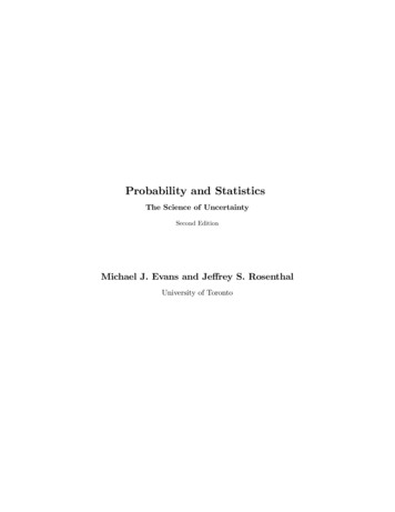
61.3CHAPTER 1. THE PROPERTIES OF MATTER IN BULKFluid StaticsI mentioned above that statistical mechanics asks questions like “How does the pressure change with volume?”. But what is pressure? Most people will answer by saying that pressure is force per area:pressure force.area(1.1)But force is a vector and pressure is a scalar, so how can this formula be correct? The aim of this section isto investigate what this formula means and find out when it is correct.21.3.1Problems1.1 (I) The rotating water glassA cylinder containing a fluid of mass density ρ is placed on the center of a phonograph turntable androtated with constant angular velocity ω. After some initial sloshing of the fluid, everything calmsdown to a steady state.ωyp p p pp p p p p p p p p p p p p p p p p p p p p p p p p p p p p p p p p66 r6hhca. The pressure is a function of height h and distance from the axis r. Show that the variation ofpressure with radial distance is p(r, h) ρω 2 r,(1.2) rwhile the variation with vertical distance is p(r, h) ρg. h(1.3)(Where g is the acceleration of gravity.)2 As such, the aim of this section is quite modest. If you want to learn more about the interesting subject of fluid flow, seethe “Resources” section of this chapter.

1.4. PHASE DIAGRAMS7b. The pressure at the surface of the fluid at the center of the cylinder (r 0, h hc ) is of courseatmospheric pressure pa . Integrate the differential equations of part (a.) to show that, at anypoint in the fluid,(1.4)p(r, h) pa 12 ρω 2 r2 ρg(h hc ).c. Show that the profile of the fluid surface is given byy(r) 1.4ω2 2r .2g(1.5)Phase DiagramsToo often, books such as this one degenerate into a study of gases. . . or even into a study of the ideal gas!Statistical mechanics in fact applies to all sorts of materials: fluids, crystals, magnets, metals, polymers,starstuff, even light. I want to show you some of the enormous variety of behaviors exhibited by matter inbulk, and that can (at least in principle) be explained through statistical mechanics.Because the axes of a phase diagram are pressure and temperature, the misconception arises that phasediagrams plot pressure as a function of temperature. No. Pressure and temperature are independent variables. For example, volume is a function of pressure and temperature, V (T, p). Instead, the lines on a phasediagram mark the places where there are cliffs in the function V (T, p).End with the high Tc phase diagram of Amnon Aharony discussed by MEF at Gibbs Symposium.Birgeneau.ResourcesThe problems of fluid flow are neglected in the typical American undergraduate physics curriculum. Anintroduction to these fascinating problems can be found in the chapters on elasticity and fluids in anyintroductory physics book, such asF.W. Sears, M.W. Zemansky, and H.D. Young, University Physics, fifth edition (Addison-Wesley,Reading, Massachusetts, 1976), chapters 10, 12, and 13, orD. Halliday, R. Resnick, and J. Walker, Fundamentals of Physics, fourth edition (John Wiley,New York, 1993), sections 16–1 to 16–7.More idiosyncratic treatments are given byR.P. Feynman, R.B. Leighton, and M. Sands, The Feynman Lectures on Physics (Addison-Wesley,Reading, Massachusetts, 1964), chapters II-40 and II-41, andJearl Walker The Flying Circus of Physics (John Wiley, New York, 1975), chapter 4.

8CHAPTER 1. THE PROPERTIES OF MATTER IN BULKHansen and McDonaldAn excellent description of various states of matter (including liquid crystals, antiferromagnets, superfluids, spatially modulated phases, and more) extending our section on “Phase Diagrams” isMichael E. Fisher, “The States of Matter—A Theoretical Perspective” in W.O. Milligan,ed., Modern Structural Methods (The Robert A. Welch Foundation, Houston, Texas, 1980) pp.74–175.1.5Additional Problems1.2 (I*) Compressibility, expansion coefficientThe “isothermal compressibility” of a substance is defined asκT (p, T ) 1 V (p, T ),V (p, T ) p(1.6)where the volume V (p, T ) is treated as a function of pressure and temperature.a. Justify the name “compressibility”. If a substance has a large κT is it hard or soft? Since “squeeze”is a synonym for “compress”, is “squeezeabilty” a synonym for “compressibility”? Why were thenegative sign and the factor of 1/V included in the definition?b. The “expansion coefficient” isβ(p, T ) V (p, T )1.V (p, T ) T(1.7)In most situations β is positive, but it can be negative. Give one such circumstance.c. What are κT and β in a region of two-phase coexistence (for example, a liquid in equilibrium withits vapor)?d. Find κT and β for an ideal gas, V (p, T ) N kB T /p.e. Show that β(p, T ) κT (p, T ) T p(1.8)for all substances.f. Verify this relation for the ideal gas. (Clue: The two expressions are not both equal to N kB /p2 V .)1.3 (I*) Heat capacity as a susceptibilityLater in this book we will find that the “heat capacity” of a fluid3 isCV (T, V, N ) 3 Technically,the “heat capacity at constant volume”. E(T, V, N ), T(1.9)

1.5. ADDITIONAL PROBLEMS9where the energy E(T, V, N ) is considered as a function of temperature, volume, and number of particles. The heat capacity is easy to measure experimentally and is often the first quantity observedwhen new regimes of temperature or pressure are explored. (For example, the first sign of superfluidHe3 was an anomalous dip in the measured heat capacity of that substance.)a. Explain how to measure the heat capacity of a gas given a strong, insulated bottle, a thermometer,a resistor, a voltmeter, an ammeter, and a clock.b. Near the superfluid transition temperature Tc , the heat capacity of Helium is given byCV (T ) A ln( T Tc /Tc ).(1.10)Sketch the heat capacity and the energy as a function of temperature in this region.c. The heat capacity is one member of a class of thermodynamic quantities called “susceptibilities”.Why does it have that name? (Clues: A change in temperature causes a change in energy, buthow much of a change? If the heat capacity is relatively high, is the system relatively sensitive orinsensitive (i.e. susceptible or insusceptible) to such temperature changes?)d. Interpret the isothermal compressibility (1.6) as a susceptibility. (Clue: A change in pressurecauses a change in volume.)1.4 (I) The meaning of “never”(This problem is modified from Kittel and Kroemer, Thermal Physics, second edition, page 53.)It has been said4 that “six monkeys, set to strum unintelligently on typewriters for millions of years,would be bound in time to write all the books in the British Museum”. This assertion gives a misleadingimpression concerning very large numbers.5 Consider the following situation: The quote considers six monkeys. Let’s be generous and allow 1010 monkeys to work. (Abouttwice the present human population.) The quote vaguely mentions “millions of years”. The age of the universe is about 14 billion years,so let’s allow all of that time, about 1018 seconds. The quote wants to write out all the books in a very large library. Let’s be modest and demandonly the production of Shakespeare’s Hamlet, a work of about 105 characters. Finally, assume that a monkey can type ten characters per second, and for definiteness, assume akeyboard of 29 characters (letters, comma, period, space. . . ignore caPitALIzaTion).a. Show that the probability that a given sequence of 105 characters comes out through a randomstriking of 105 keys is1 10 146 240 .(1.11)10029 000How did you perform the arithmetic?4 J.Jeans, Mysterious Universe (Cambridge University Press, Cambridge, 1930) p. 4.insightful discussion of the “monkeys at typewriters” problem, and its implications for biological evolution, is given byRichard Dawkins in his book The Blind Watchmaker (Norton, New York, 1987) pp. 43–49.5 An

10CHAPTER 1. THE PROPERTIES OF MATTER IN BULKb. Show that the probability of producing Hamlet through the “unintelligent strumming” of 1010monkeys over 1018 seconds is about 10 146 211 , which is small enough to be considered zero formost purposes.1.5 Human geneticsThere are about 21,000 genes in the human genome. Suppose that each gene could have any of threepossible states (called “alleles”). (For example, if there were a single gene for hair color, the threealleles might be black, brown, and blond.) Then how many genetically distinct possible people wouldthere be? Compare to the current worldwide human population. Estimate how long it would takefor ever

Statistical mechanics treats matter in bulk. While most branches of physics.classical mechanics, atomic physics, quantum mechanics, nuclear physics.deal with one or two or a few dozen particles, statistical mechanics deals with, typically, about a