Transcription
Computational Fluid DynamicsIntroduction!Computational Fluid DynamicsIntroduction!What is ComputationalFluid Dynamics (CFD)?!Finite Difference or!Finite Volume Grid!Computational Fluid DynamicsIntroduction!Computational Fluid DynamicsIntroduction!Using CFD to solve a problem:!Preparing the data (preprocessing):!Setting up the problem, determining flowparameters and material data andgenerating a grid.!Grid must besufficiently fine toresolve the flow!Solving the problem!Analyzing the results (postprocessing):Visualizing the data and estimatingaccuracy. Computing forces and otherquantities of interest. !Computational Fluid DynamicsIntroduction!CFD is an interdisciplinary topic!Numerical!Fluid!Analysis! mputational Fluid DynamicsIntroduction!Many website contain information about fluiddynamics and computational fluid dynamicsspecifically. Those include!!NASA site with CFD FD Online: An extensive collection ofinformation but not always very m is a monitored site with a largenumber of fluid mechanics material!http://www.e-fluids.com/!
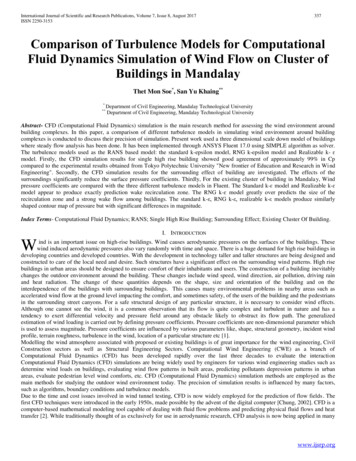
Computational Fluid DynamicsComputational Fluid DynamicsBeginning of CFD!CFD at Los AlamosThe MANIAC at Los Alamos had already stimulated considerableinterest in numerical solutions at the Laboratory. However, CFD in themodern sense started with the formation of the T3 group. Earlydevelopment in the Group focused on:Beginning ofCFD!Compressible flows: Particles in Cells (1955): Eularian –Lagrangianmethod where particles move through a fixed gridLow-speed (incompressible) flowsVorticity streamfunction for homogeneous(mostly 2D) flows (1963)Marker and Cell for free surface andMultiphase flows in primitive variables (1965)All-speed flows—ICE (1968, 1971)Arbitrary–Lagrangian–Eulerian (ALE) methodsComputational Fluid DynamicsBeginning of CFD!Computational Fluid DynamicsBeginning of CFD!Incompressible flows—Vorticity-Streamfunction MethodIncompressible flows—the MAC MethodPrimitive variables (velocity and pressure) on a staggeredgridpi-1,j 1pi-1,jThe velocity is updated using splitting where we first ignorepressure and then solve a pressure equation with thedivergence of the predicted velocity as a source termMarker particles used to track the different fluidsComputations of the development of a von Karman vortex streetbehind a blunt body by the method developed by J. Fromm. Timegoes from left to right showing the wake becoming unstable.From: J. E. Fromm and F. H. HarIow, Numerical Solution of theProblem of Vortex Street Development: Phys. Fluids 6 (1963), 975.Computational Fluid DynamicsBeginning of CFD!Early Publicity: Science MagazineF.H. Harlow, J.P. Shannon,Distortion of a splashing liquiddrop, Science 157 (August)(1967) 547–550.pi-1,j-1pi,j 1ui 1/2,j 1ui-1/2,jpi,jui 1/2,jpi,j-1pi 1,jvi 1,j-1/2vi,j-1/2ui-1/2,j-1pi 1,j 1vi 1,j 1/2vi,j 1/2vi-1,j-1/2ui 1/2,j-1pi 1,j-1The dam breaking problemsimulated by the MACmethod, assuming a freesurface. From F. H. Harlowfig1.pdfand J. E. Welch. Numericalcalculation of timedependent viscousincompressible flow of fluidwith a free surface. Phys.Fluid, 8: 2182–2189, 1965.Computational Fluid DynamicsBeginning of CFD!F.H. Harlow, J.P.Shannon, J.E.Welch, Liquid wavesby computer,Science 149(September) (1965)1092–1093.ui-1/2,j 1vi-1,j 1/2
Computational Fluid DynamicsBeginning of CFD!“While most of the scientific and technological world maintained adisdainful distaste (or at best an amused curiosity) for computing, thepower of the stored-program computers came rapidly into its own at LosAlamos during the decade after the War.”From: Computing & Computers: Weapons Simulation Leads to theComputer Era, by Francis H. Harlow and N. Metropolis“Another type of opposition occurred in our interactions with editors ofprofessional journals, and with scientists and engineers at various universitiesand industrial laboratories. One of the things we discovered in the 1950s andearly 1960s was that there was a lot of suspicion about numerical techniques.Computers and the solutions you could calculate were said to be theplaythings of rich laboratories. You couldnʼt learn very much unless you didstudies analytically.“From: Journal of Computational Physics 195 (2004) 414–433Review: Fluid dynamics in Group T-3 Los Alamos National Laboratory(LA-UR-03-3852), by Francis H. HarlowComputational Fluid DynamicsBeginning of CFD!Computational Fluid DynamicsBeginning of CFD!CFD goes mainstreamEarly studies using the MAC method:R. K.-C. Chan and R. L. Street. A computer study of finite-amplitudewater waves. J. Comput. Phys., 6:68–94, 1970.G. B. Foote. A numerical method for studying liquid drop behavior:simple oscillations. J. Comput. Phys., 11:507–530, 1973.G. B. Foote. The water drop rebound problem: dynamics of collision.J. Atmos. Sci., 32:390–402, 1975.R. B. Chapman and M. S. Plesset. Nonlinear effects in the collapse ofa nearly spherical cavity in a liquid. Trans. ASME, J. Basic Eng.,94:142, 1972.T. M. Mitchell and F. H. Hammitt. Asymmetric cavitation bubblecollapse. Trans ASME, J. Fluids Eng., 95:29, 1973.Beginning of commercial CFD—Imperial College (Spalding)Computations in the Aerospace Industry (Jameson and others)And others!Computational Fluid DynamicsBeginning of CFD!Although the methods developed at Los Alamos were put to use in solvingpractical problems and picked up by researchers outside the Laboratory,considerable development took place that does appear to be only indirectlymotivated by it. Those development include:Panel methods for aerodynamic computations (Hess and Smith, 1966)Specialized techniques for free surface potential and stokes flows (1976)and vortex methodsThe development of computer fluid dynamics has been closely associated with the evolutionof large high-speed computers. At first the principal incentive was to produce numericaltechniques for solving problems related to national defense. Soon, however, it wasrecognized that numerous additional scientific and engineering applications could beaccomplished by means of modified techniques that extended considerably the capabilities ofthe early procedures. This paper describes some of this work at The Los Alamos NationalLaboratory, where many types of problems were solved for the first time with the newlyemerging sequence of numerical capabilities. The discussions focus principally on those withwhich the author has been directly involved.Computational Fluid DynamicsCommercialCodes!Spectral methods for DNS of turbulent flows (late 70ʼs, 80ʼs)Monotonic advection schemes for compressible flows (late 70ʼs, 80ʼs)Steady state solutions (SIMPLE, aeronautical applications, etc)Commercial CFDHowever, with outside interest in Multifluid simulations (improved VOF, levelsets, front tracking) around 1990, the legacy became obviousComputational Fluid DynamicsCommercial Codes!CHAM (Concentration Heat And Momentum) founded in 1974by Prof. Brian Spalding was the first provider of generalpurpose CFD software. The original PHOENICS appeared in1981.!!The first version of the FLUENT code was launched inOctober 1983 by Creare Inc. Fluent Inc. was established in1988.!!STAR-CD's roots go back to the foundation of ComputationalDynamics in 1987 by Prof. David Gosman,!!The original codes were relatively primitive, hard to use, andnot very accurate.!
Computational Fluid DynamicsCommercial Codes!Computational Fluid DynamicsCommercial Codes!What to expect and when to use commercial package:!!The current generation of CFD packages generally iscapable of producing accurate solutions of simple flows.The codes are, however, designed to be able to handlevery complex geometries and complex industrialproblems. When used with care by a knowledgeable userCFD codes are an enormously valuable design tool. !!Commercial CFD codes are rarely useful for state-of-theart research due to accuracy limitations, the limitedaccess that the user has to the solution methodology, andthe limited opportunities to change the code if needed !Major current players include!!Ansys (Fluent and other m/!!adapco: ttp://www.cham.co.uk/CFD2000: !http://www.adaptive-research.com/Computational Fluid Dynamicshttp://www.nd.edu/ gtryggva/CFD-Course/!A Finite Difference Codefor the Navier-StokesEquations in Vorticity/Streamfunction!Form!Computational Fluid DynamicsThe vorticity/streamfunction equations:!!" !u!u!u! p 1 # ! 2u ! 2u & u v " !x!y! x Re % ! x 2 ! y 2 ('"y ! t!v!v! p 1 # ! 2v ! 2v &! !v u v " !t!x!y! y Re % ! x 2 ! y 2 ('!x!"!"!"1 #% ! 2 " ! 2" & u v !t!x!y Re !x 2 !y 2 '! where!Computational Fluid DynamicsObjectives!Defining the streamfunction by!u !"!"; v #!y!xAnd substituting into the definition of the vorticity!! "v "u#"x "ygives!! 2" ! 2" # ! x2 ! y2" v "u#"x " yComputational Fluid DynamicsThe vorticity/streamfunction equations:!The system to be solved is the Navier-Stokesequations in vorticity-stream function form are:!Advection/diffusion equation!!"! !" ! !"1 % ! 2" ! 2" ( # !t! y ! x ! x ! y Re '& ! x 2 ! y 2 *)Elliptic equation!! 2" ! 2" # ! x2 ! y2where!u !"!"; v #!y!x
Computational Fluid DynamicsFinite Difference Approximations!Computational Fluid DynamicsFinite Difference Approximations!Notation: the location of variables on a structured grid!(x, y)f i, j f (x, y)f i, j 1j 1f i!1, j f i, jjf i 1, ji -1if i!1, j f (x ! h, y)f i, j 1 f (x, y h)f i, j !1j-1f i 1, j f (x h, y)i 1Then we replace the equations at each grid pointby a finite difference approximation!nn! 2 f (x) f (x h) " 2 f (x) f (x " h) ! 4 f (x) h2 " !! x2h2! x 4 xx! f (t) f (t "t) # f (t) ! 2 f (t) "t # !!t"t!t 2 2Computational Fluid DynamicsFinite Difference Approximations!!"! !" ! !"1 % ! 2" ! 2" ( # !t! y ! x ! x ! y Re '& ! x 2 ! y 2 *)The advection equation is:!!n 1i, j" ! i,n j #tnnnn% i,n j 1 " i,n j "1 ( % ! i 1,( % i 1,( % ! i,n j 1 " ! i,n j "1 (" ! i"1," i"1,jjjj"'*'* '*'*2h2h2h2h&)&) &)&) nnnnn1 % ! i 1, j ! i"1, j ! i, j 1 ! i, j "1 " 4! i, j ('*2Re &h)n! 2" #%! 2" # 2 % &' i,n j2!x i, j !y i, jComputational Fluid DynamicsFinite Difference Approximations!! f (x) f (x h) " f (x " h) ! 3 f (x) h2 " !!x2h! x 3 12nnf i, j !1 f (x, y ! h)Finite difference approximations!n!" #!& !" #!& !" #1 ') ! 2" ! 2" #* % !t i, j!y !x i, j !x !y i, j Re ( !x 2 !y 2 i, jComputational Fluid DynamicsFinite Difference Approximations!Laplacian!!2 f ! 2 f !x 2 !y 2nfi n 1, j ! 2 fi,nj fi!1,f n ! 2 f i,nj fi n, j !1j i, j 1 2hh2fi n 1, j fin!1 , j fi,nj 1 fi n, j !1 ! 4 fi n, j2hComputational Fluid DynamicsFinite Difference Approximations!The vorticity at the new time is given by:! % n # n ( %!n #!n (i, j 1i, j #1i 1, ji#1, j! i,n 1 ! i,n j "t - # '*'*j2h2h-, &)&)nn% i 1,( % ! i,n j 1 # ! i,n j #1 (# i#1,jj '*'*2h2h&)&) nnnnn1 % ! i 1, j ! i#1, j ! i, j 1 ! i, j #1 # 4! i, j ( .'*0Re &h2) 0/
! 2" ! 2" # ! x2 ! y2nn! i 1, ! i"1, ! i,n j 1 ! i,n j "1 " 4! i,n jjjh2 "# i,n jThe Driven Cavity Problem!!We will now use thisapproach to solve for the flowin a driven cavity. The drivencavity is a square domainwith a moving wall at the topand stationary side andbottom walls. The simplegeometry and the absence ofin and outflow makes this aparticularly simple andpopular test problem.!Computational Fluid DynamicsBoundary Conditions for the Streamfunction!Moving wall!Stationary wall!The elliptic equation is:!Computational Fluid DynamicsThe Driven Cavity Problem!Stationary wall!Computational Fluid DynamicsFinite Difference Approximations!Stationary wall!Computational Fluid DynamicsDiscretizing the Domain!To compute an approximate solution numerically,we start by laying down a discrete grid:!Since the boundariesmeet, the constantmust be the same onall boundaries!j NY!! i, j and " i , jGridboundariescoincidewith domainboundaries!stored ateach gridpoint!! Constantj 2!j 1!i 1! i 2!Computational Fluid DynamicsFinite Difference Approximations!These equations allow us to obtain the solution atinterior points!! i, j 0j ny!on the boundary!Need vorticityon theboundary!!i NX!Computational Fluid DynamicsBoundary Conditions for the Streamfunction!To update the vorticity in the interior of the domain, we needthe vorticity at the wall. Once the streamfunction (and thus thevelocity) everywhere has been found, this can be done. !!At the bottom wall:!! "v "u"u! !"x " y"ySince the normalvelocity is zero!Where the velocity can be found from the streamfunction!j 2!j 1!i 1! i 2!i nx!u !"!y
Computational Fluid DynamicsDiscrete Boundary Condition!Consider the bottom wall (j 1):!Need to find! ! wallThe elliptic equation:! ! i, j 1The velocity at j 3/2 can be foundby centered differences:!j 3j 2j 1u(i, 23 ) Uwalli -1ii 1Similar expressionscan be found forthe other walls!Computational Fluid DynamicsSolving the elliptic equation!!" " (i,2) " (i,1)#!yhThe vorticity is then found byone-sided differences!# u u(i, 23 ) " u(i,1) #yh/2)"2 & % (i,2) " % (i,1) " U wall h '(h*! (i,1) "! in 1, j ! in"1, j ! ni, j 1 ! ni, j "1 " 4! i,n j "# i,n jh2Rewrite as!nnnn2 n! i,n 1j 0.25 (! i 1, j ! i"1, j ! i, j 1 ! i, j "1 h # i, j )Solve by SOR!2 n! "i, j 1 # 0.25 (! "i 1, j ! "i 1, 1j !i," j 1 ! "i, 1j 1 h % i, j ) (1 # )! "i, jComputational Fluid DynamicsSolution Strategy!Limitations on thetime step!! "t 1#h24( u v )!t#2"Computational Fluid DynamicsSolution Strategy!Initial vorticity given!Initial vorticity given!Solve for the stream function!Solve for the stream function!Find vorticity on boundary!Find vorticity on boundary!Find RHS of vorticity equation!Find RHS of vorticity equation!Update vorticity in interior!Update vorticity in interior!t t dt!t t !t!Computational Fluid DynamicsThe clf;nx 9; ny 9; MaxStep 60; Visc 0.1; dt 0.02;% resolution & governing parametersMaxIt 100; Beta 1.5; MaxErr 0.001;% parameters for SOR iterationsf zeros(nx,ny); vt zeros(nx,ny); w zeros(nx,ny); h 1.0/(nx-1); t 0.0;for istep 1:MaxStep,% start the time integrationfor iter 1:MaxIt,% solve for the streamfunctionw sf;% by SOR iterationfor i 2:nx-1; for j 2:ny-1sf(i,j) 0.25*Beta*(sf(i 1,j) sf(i-1,j). sf(i,j 1) sf(i,j-1) h*h*vt(i,j)) (1.0-Beta)*sf(i,j);end; end;Err 0.0; for i 1:nx; for j 1:ny, Err Err abs(w(i,j)-sf(i,j)); end; end;if Err MaxErr, break, end% stop if iteration has convergedend;vt(2:nx-1,1) -2.0*sf(2:nx-1,2)/(h*h);% vorticity on bottom wallvt(2:nx-1,ny) -2.0*sf(2:nx-1,ny-1)/(h*h)-2.0/h;% vorticity on top wallvt(1,2:ny-1) -2.0*sf(2,2:ny-1)/(h*h);% vorticity on right wallvt(nx,2:ny-1) -2.0*sf(nx-1,2:ny-1)/(h*h);% vorticity on left wallfor i 2:nx-1; for j 2:ny-1% computew(i,j) -0.25*((sf(i,j 1)-sf(i,j-1))*(vt(i 1,j)-vt(i-1,j)).% the RHS-(sf(i 1,j)-sf(i-1,j))*(vt(i,j 1)-vt(i,j-1)))/(h*h).% of the Visc*(vt(i 1,j) vt(i-1,j) vt(i,j 1) vt(i,j-1)-4.0*vt(i,j))/(h*h); % vorticityend; end;% equationvt(2:nx-1,2:ny-1) vt(2:nx-1,2:ny-1) dt*w(2:nx-1,2:ny-1);% update the vorticityt t dt% print out tsubplot(121), contour(rot90(fliplr(vt))), axis('square');% plot vorticitysubplot(122), contour(rot90(fliplr(sf))), axis('square');pause(0.01) % streamfunctionend;For l 1:MaxIterations!for i 2:nx-1; for j 2:ny-1!s(i,j) SOR for the stream function!end; end!end!v(i,j) !for i 2:nx-1; for j 2:ny-1!rhs(i,j) Advection diffusion!end; end!v(i,j) v(i,j) dt*rhs(i,j)!Computational Fluid DynamicsResults:!17 by 17!Dt 0.01!D 0.1!
Computational Fluid DynamicsResults:!Vorticity!Computational Fluid DynamicsResults:!17 by 17!Dt 0.01!D 02015201510105015201510105550009 by 9 grid!17 by 17 grid!Computational Fluid DynamicsResults:!Vorticity!!" " i, j 1 "i, j 1#!y2h" i 1, j " i 1, j!"v i, j # !x2hui, j 0.040Streamfunction!Computational Fluid DynamicsIN/OUT FLOW!The driven cavity problem is particularly simple sincethere is no in or out flow. In the streamfunction-vorticityform of the Navier-Stokes equations it is, however,relatively easy to include specified in and outflow.!!An inflow through the right horizontal wall, for example,can be imposed by increasing the streamfunctionbetween each grid point by:! !" u!y!For incompressible flow the inflow must matched byoutflow and if we specify the outflow velocity the thestreamfunction must be decreased by the same amountelsewhere on the boundary!
Computational Fluid Dynamics! Numerical ! Analysis !!!!! Fluid Mechanics! CFD!!!!! Computer! Science! CFD is an interdisciplinary topic! Introduction! Computational Fluid Dynamics! Many website contain information about fluid dynamics and computational fluid dynamics specifically. Th