Transcription
2.29 Numerical Fluid MechanicsSpring 2015 – Lecture 22REVIEW Lecture 21: Time-Marching Methods and ODEs – IVPs: End– Multistep/Multipoint Methods: Adams Methods Additional points are at past time steps– Practical CFD Methods– Implicit Nonlinear systems– Deferred-correction Approach Complex Geometries– Different types of grids– Choice of variable arrangements: Grid Generation– Basic concepts and structured grids Stretched grids Algebraic methods (for stretched grids), Transfinite Interpolation2.29Numerical Fluid MechanicsPFJL Lecture 22,1
TODAY (Lecture 22):Grid Generation and Intro. to Finite Elements Grid Generation– Basic concepts and structured grids, cont’d General coordinate transformation Differential equation methods Conformal mapping methods– Unstructured grid generation Delaunay Triangulation Advancing Front method Finite Element Methods– Introduction– Method of Weighted Residuals: Galerkin, Subdomain and Collocation– General Approach to Finite Elements: Steps in setting-up and solving the discrete FE system Galerkin Examples in 1D and 2D– Computational Galerkin Methods for PDE: general case Variations of MWR: summary Finite Elements and their basis functions on local coordinates (1D and 2D)2.29Numerical Fluid MechanicsPFJL Lecture 22,2
References and Reading AssignmentsComplex Geometries and Grid Generation Chapter 8 on “Complex Geometries” of “J. H. Ferziger and M.Peric, Computational Methods for Fluid Dynamics. Springer,NY, 3rd edition, 2002” Chapter 9 on “Grid Generation” of T. Cebeci, J. P. Shao, F.Kafyeke and E. Laurendeau, Computational Fluid Dynamics forEngineers. Springer, 2005. Chapter 13 on “Grid Generation” of Fletcher, ComputationalTechniques for Fluid Dynamics. Springer, 2003. Ref on Grid Generation only:– Thompson, J.F., Warsi Z.U.A. and C.W. Mastin, “Numerical GridGeneration, Foundations and Applications”, North Holland, 19852.29Numerical Fluid MechanicsPFJL Lecture 22,3
Grid Generation for Structured Grids:General Coordinate transformation For structured grids, mapping of coordinates fromCartesian domain to physical domain is defined by x a transformation: xi xi ( ξj ) (i & j 1, 2, 3)J det i All transformations are characterized by theirJacobian determinant J. j x1 1 x1 2 x1 3 x2 1 x2 2 x2 3 x3 1 x3 3 x3 3– For Cartesian vector components, one only needs to transformderivatives. One has: j ij x , where ij represents the cofactor of i (element i, j of Jacobian matrix) xi j xi j J j– In 2D, x x (ξ,η) and (ξ,η), this leads to: 11 12 1 y y x x x J JJ Recall: the minor element mij corresponding to aij is the determinant of the submatrix that remainsafter the ith row and the jth column are deleted from A. The cofactor cij of aij is: cij ( 1)i j mij2.29Numerical Fluid MechanicsPFJL Lecture 22,4
Grid Generation for Structured Grids:General Coordinate transformation, Cont’d How do the conservation equations transform?The generic conservation equation in Cartesian coordinates: . ( v ) . (k ) s t becomes:where:J v j k s t x j x j k mj B J s U j t j J m U j vk kj v1 1 j v2 2 j v3 3 j source unknown. All rights reserved.This contentis excluded from our CreativeCommons license. For more information,see http://ocw.mit.edu/help/faq-fair-use/.is proportional to the velocity component aligned with j(normal to j const.)B mj kj km 1 j 1m 2 j 2m 3 j 3m are coefficients, sum of products of cofactors ij As a result, each 1st derivative term is replaced by a sum of three termswhich contains derivatives of the coordinates as coefficients Unusual features of conservation equations in non-orthogonal grids:– Mixed derivatives appear in the diffusive terms and metrics coefficients appearin the continuity eqn.2.29Numerical Fluid MechanicsPFJL Lecture 22,5
Structured Grids: Gen. Coord. transformation, Cont’dSome Comments Coordinate transformation often presented only as a meansof converting a complicated non-orthogonal grid into asimple, uniform Cartesian grid (the computational domain,whose grid-spacing is arbitrary) However, simplification is only apparent:– Yes, the computational grid is simpler than the original physical one– But, the information about the complexity in the computational domainis now in the metric coefficients of the transformed equations i.e. discretization of computational domain is now simple, but thecalculation of the Jacobian and other geometric information is not trivial(the difficulty is hidden in the metric coefficients) As mentioned earlier, FD method can in principle be appliedto unstructured grids: specify a local shape function, differentiate andwrite FD equations. Has not yet been done.2.29Numerical Fluid MechanicsPFJL Lecture 22,6
Grid Generation for Structured Grids:Differential Equation Methods Grid transformation relations determined by a finite-differencesolution of PDEs– For 2D problems, two elliptic (Poisson) PDEs are solved– Can be done for any coordinate systems, but here we will use Cartesiancoordinates. The 2D transformation is then: From the physical domain (x, y) to the computational domain (ξ, η) At physical boundaries, one of ξ, η is constant, the other is monotonically varying At interior points: 2 2 P( , ) x 2 y 2 2 2 Q ( , ) x 2 y 2where P( , ) and Q( , ) are called the “control functions” Their selection allows to concentrate the ξ, η lines in specific regions If they are null, coordinates will tend to be equally spaced away from boundaries Boundary conditions: ξ, η specified on boundaries of physical domain2.29Numerical Fluid MechanicsPFJL Lecture 22,7
Grid Generation for Structured Grids:Differential Equation Methods, Cont’d Computations to generate the grid mapping are actually carriedout in the computational domain (ξ, η) itself !– don’t want to solve the elliptic problem in the complex physical domain! Using the general rule, the elliptic problem is transformed into: 2 x 2 x 2 x x x 2 2 2 JP Q 0 2 2 y 2 y 2 y y y 2 2 2 JP Q 0 2 where x 2 y 2 ; x x y y ; x 2 y 2 ; J x y x y (with x x, etc) – Boundary conditions are now the transformed values of the BCs in (x, y)domain: they are the values of the positions (x, y) of the grid points on thephysical domain mapped to their locations in the computational domain– Equations can be solved by FD method to determine values of every gridpoint (x, y) in the interior of the physical domain Method developed by Thomson et al., 1985 (see ref)2.29Numerical Fluid MechanicsPFJL Lecture 22,8
Grid Generation for Structured Grids:Differential Equation Methods, Example Springer. All rights reserved. This content is excluded from our CreativeCommons license. For more information, see http://ocw.mit.edu/fairuse.2.29Numerical Fluid MechanicsPFJL Lecture 22,9
Grid Generation for Structured Grids:Conformal Mapping Methods Conformal mapping schemes are analytical or partially analytical (asopposed to differential equation methods) Restricted to two dimensional flows (based on complex variables): useful forairfoils Examples: Springer. All rights reserved. This content is excluded from our CreativeCommons license. For more information, see http://ocw.mit.edu/fairuse.– C-mesh: high density near leading edge of airfoil and good wake– O-mesh: high density near leading and trailing edge of airfoil– H-mesh: two sets of mesh lines similar to a Cartesian mesh, which is easiest togenerate. Its mesh lines are often well aligned with streamlines2.29Numerical Fluid MechanicsPFJL Lecture 22,10
Grid Generation for Structured Grids:Conformal Mapping Methods: Example C-mesh example is generated by a parabolic mapping function It is essentially a set of confocal, orthogonal parabolas wrapping around theairfoil The mapping is defined by:2( x iy ) ( i ) 2or2 x 2 2 ;y Inverse transformation: 2 x2 y 2 x ; 2 x2 y 2 x Springer. All rights reserved. This content is excluded from our CreativeCommons license. For more information, see http://ocw.mit.edu/fairuse. Polar coordinates can be used for easier “physical plane” to “computationalplane” transformation. In conformal mapping, singular point is point where mapping fails (here, it isthe origin) move it to half the distance from the nose radius2.29Numerical Fluid MechanicsPFJL Lecture 22,11
Grid Generation: Unstructured Grids Generating unstructured grid iscomplicated but now relativelyautomated in “classic” cases Involves succession of smoothingtechniques that attempt to alignelements with boundaries of physicaldomain Decompose domain into blocks to decouple the problems Need to define point positions andconnections Most popular algorithms:– Delaunay Triangulation Method Springer. All rights reserved. This content is excluded from our CreativeCommons license. For more information, see http://ocw.mit.edu/fairuse.– Advancing Front Method Two schools of thought: structured vs.unstructured, what is best for CFD?2.29– Structured grids: simpler grid and straightforwardtreatment of algebraic system, but mesh generationconstraints on complex geometries– Unstructured grids: generated faster on complexdomains, easier mesh refinements, but data storageand solution of algebraic system more complexNumerical Fluid MechanicsPFJL Lecture 22,12
Grid Generation: Unstructured Grids– This geometrical construction is known as theDirichlet (Voronoi) tessellation Delaunay Triangulation (DT)–Use a simple criterion to connect points toform conforming, non-intersecting elements–Maximizes minimum angle in each triangle–Not unique–Task of point generation is doneindependently of connection generation Based on Dirichlet’s domaindecomposition into a set of packedconvex regions:–For a given set of points P, the space issubdivided into regions in such a way thateach region is the space closer to P than toany other point Dirichlet tessellation– The sides of the polygon around P is made ofsegments bisectors of lines joining P to itsneighbors: if all pair of such P points with acommon segment are joined by straight lines,the result is a Delaunay Triangulation– Each vortex of a Voronoi diagram is then thecircumcenter of the triangle formed by thethree points of a Delaunay triangle– Criterion: the circumcircle can not contain anyother point than these three points215– The tessellation of a closed domain results ina set of non-overlapping convex regions calledVoronoi regions/polygonsP43Note: at the end,points P are atsummits of triangles(a) Satisfies the criterionImage by MIT OpenCourseWare.2.29(b)boes notImage by MIT OpenCourseWare.Numerical Fluid MechanicsPFJL Lecture 22,13
Grid Generation: Unstructured Grids Advancing Front Method– In this method, the tetrahedras are built progressively, inward from theboundary– An active front is maintained where new tetrahedra are formed– For each triangle on the edge of the front, an ideal location for a newthird node is computed– Requires intersection checks to ensure triangles don’t overlap Springer. All rights reserved. This content is excluded from our CreativeCommons license. For more information, see http://ocw.mit.edu/fairuse. In 3D, the Delaunay Triangulation is preferred (faster)2.29Numerical Fluid MechanicsPFJL Lecture 22,14
References and Reading AssignmentsFinite Element Methods Chapters 31 on “Finite Elements” of “Chapra and Canale,Numerical Methods for Engineers, 2006.” Lapidus and Pinder, 1982: Numerical solutions of PDEs inScience and Engineering. Chapter 5 on “Weighted Residuals Methods” of Fletcher,Computational Techniques for Fluid Dynamics. Springer, 2003. Some Refs on Finite Elements only:– Hesthaven J.S. and T. Warburton. Nodal discontinuous Galerkinmethods, vol. 54 of Texts in Applied Mathematics. Springer, New York,2008. Algorithms, analysis, and applications– Mathematical aspects of discontinuous Galerkin methods (Di Pietroand Ern, 2012)– Theory and Practice of Finite Elements (Ern and Guermond, 2004)2.29Numerical Fluid MechanicsPFJL Lecture 22,15
FINITE ELEMENT METHODS: Introduction Finite Difference Methods: based on a discretization of the differential formof the conservation equations– Solution domain divided in a grid of discrete points or nodes– PDE replaced by finite-divided differences “point-wise” approximation– Harder to apply to complex geometries Finite Volume Methods: based on a discretization of the integral forms of theconservation equations:– Grid generation: divide domain into set of discrete control volumes (CVs)– Discretize integral equation– Solve the resultant discrete volume/flux equations Finite Element Methods: based on reformulation of PDEs into minimizationproblem, pre-assuming piecewise shape of solution over finite elements– Grid generation: divide the domain into simply shaped regions or “elements”– Develop approximate solution of the PDE for each of these elements– Link together or assemble these individual element solutions, ensuring somecontinuity at inter-element boundaries PDE is satisfied in piecewise fashion2.29Numerical Fluid MechanicsPFJL Lecture 22,16
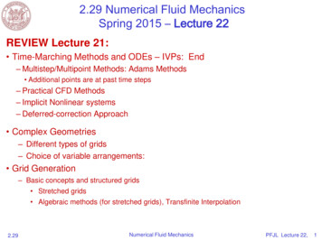
Finite Elements: Introduction, Cont’d Originally based on the Direct Stiffness Method (Navier in 1826) andRayleigh-Ritz, and further developed in its current form in the 1950’s(Turner and others) Can replace somewhat “ad-hoc” integrations of FV with more rigorousminimization principles Originally more difficulties with convection-dominated (fluid) problems,applied to solids with diffusion-dominated propertiesComparison of FD and FE gridsExamples of Finite elementsTriangularelementQuadrilateralelementLine elementNodal xahedronelementThree-dimensionalImage by MIT OpenCourseWare. McGraw-Hill. All rights reserved. This content is excluded from our Creative Commonslicense. For more information, see http://ocw.mit.edu/fairuse.2.29Numerical Fluid MechanicsPFJL Lecture 22,17
Finite Elements: Introduction, Cont’d Classic example: Rayleigh-Ritz / Calculus of variations– Finding the solution of 2u f2 xon 0,1 1is the same as finding u that minimizes J (u) 0– R-R approximation:21 u u f dx2 x n Expand unknown u into shape/trial functionsu( x ) ai i ( x )and find coefficients ai such that J(u) is minimizedi 1 Finite Elements:– As Rayleigh-Ritz but choose trial functions to be piecewise shapefunction defined over set of elements, with some continuity acrosselements2.29Numerical Fluid MechanicsPFJL Lecture 22,18
Finite Elements: Introduction, Cont’dMethod of Weigthed Residuals There are several avenues that lead to the same FEformulation– A conceptually simple, yet mathematically rigorous, approach is theMethod of Weighted Residuals (MWR)– Two special cases of MWR: the Galerkin and Collocation Methods In the MWR, the desired function u is replaced by a finiteseries approximation into shape/basis/interpolation functions:nu( x ) ai i ( x )i 1– i (x) chosen such they satisfy the boundary conditions of the problem– But, they will not in general satisfy the PDE: L u f they lead to a residual:L u ( x ) f ( x ) R( x ) 0– The objective is to select the undetermined coefficients ai so that thisresidual is minimized in some sense2.29Numerical Fluid MechanicsPFJL Lecture 22,19
Finite Elements:Method of Weigthed Residuals, Cont’d– One possible choice is to set the integral of the residual to be zero. Thisonly leads to one equation for n unknowns Introduce the so-called weighting functions wi (x) i 1,2, , n, and set theintegral of each of the weighted residuals to zero to yield n independentLequations: R( x) wi ( x) dx dt 0, i 1,2,., n– In 3D, this becomes:t 0 R(x) w (x) dx dt 0,ii 1,2,., nt V A variety of FE schemes arise from the definition of theweighting functions and of the choice of the shape functions– Galerkin: the weighting functions are chosen to be the shape functions(the two functions are then often called basis functions or test functions)– Subdomain method: the weighting function is chosen to be unity in thesub-region over which it is applied– Collocation Method: the weighting function is chosen to be a Dirac-delta2.29Numerical Fluid MechanicsPFJL Lecture 22,20
Finite Elements:Method of Weigthed Residuals, Cont’d Galerkin: R(x) (x) dx dt 0,ii 1,2,., nt V– Basis functions formally required tobe complete set of functions– Can be seen as “residual forced tozero by being orthogonal to all basisfunctions” Subdomain method: R(x) dx dt 0,i 1,2,., nt Vi– Non-overlapping domains Vi oftenset to elements– Easy integration, but not as accurate Collocation Method: R(x) x (x) dx dt 0,t Vi John Wiley & Sons. All rights reserved. This contentis excluded from our Creative Commons license. Formore information, see http://ocw.mit.edu/fairuse.i 1, 2,., n– Mathematically equivalent to say that each residual vanishes at eachcollocation points xi Accuracy strongly depends on locations xi .– Requires no integration.2.29Numerical Fluid MechanicsPFJL Lecture 22,21
MIT OpenCourseWarehttp://ocw.mit.edu2.29 Numerical Fluid MechanicsSpring 2015For information about citing these materials or our Terms of Use, visit: http://ocw.mit.edu/terms.
2.29 Numerical Fluid Mechanics PFJL Lecture 22, 11 Grid Generation for Structured Grids: Conformal Mapping Methods: Example C-mesh example is generated by a parabolic mapping function It is essentially a set of confocal, orthogonal parabolas wrapping around the airfoil The mapping is defined by: Inverse transformation: