Transcription
SOIL, 5, 107–119, 2019https://doi.org/10.5194/soil-5-107-2019 Author(s) 2019. This work is distributed underthe Creative Commons Attribution 4.0 License.SOILMulti-source data integration for soilmapping using deep learningAlexandre M. J.-C. Wadoux1 , José Padarian2 , and Budiman Minasny21 SoilGeography and Landscape Group, Wageningen University & Research, Wageningen, the Netherlands2 Sydney Institute of Agriculture, the University of Sydney, Sydney, AustraliaCorrespondence: Alexandre M. J.-C. Wadoux (alexandre.wadoux@wur.nl)Received: 29 October 2018 – Discussion started: 16 November 2018Revised: 8 February 2019 – Accepted: 7 March 2019 – Published: 22 March 2019Abstract. With the advances of new proximal soil sensing technologies, soil properties can be inferred by avariety of sensors, each having its distinct level of accuracy. This measurement error affects subsequent modelling and therefore must be integrated when calibrating a spatial prediction model. This paper introduces a deeplearning model for contextual digital soil mapping (DSM) using uncertain measurements of the soil property.The deep learning model, called the convolutional neural network (CNN), has the advantage that it uses as inputa local representation of environmental covariates to leverage the spatial information contained in the vicinity ofa location. Spatial non-linear relationships between measured soil properties and neighbouring covariate pixelvalues are found by optimizing an objective function, which can be weighted with respect to a measurement errorof soil observations. In addition, a single model can be trained to predict a soil property at different soil depths.This method is tested in mapping top- and subsoil organic carbon using laboratory-analysed and spectroscopically inferred measurements. Results show that the CNN significantly increased prediction accuracy as indicatedby the coefficient of determination and concordance correlation coefficient, when compared to a conventionalDSM technique. Deeper soil layer prediction error decreased, while preserving the interrelation between soilproperty and depths. The tests conducted suggest that the CNN benefits from using local contextual information up to 260 to 360 m. We conclude that the CNN is a flexible, effective and promising model to predict soilproperties at multiple depths while accounting for contextual covariate information and measurement error.1IntroductionDigital soil mapping (DSM) techniques are commonly usedto predict a soil property at unsampled locations using measurements at a finite number of spatial locations. Predictionis routinely done by exploiting the relationship between asoil property and one or several environmental covariates,which are assumed to represent soil forming factors. Examples of covariates are the digital elevation model (DEM) or itsderivatives (Moore et al., 1993). Demattê et al. (2018) usedmulti-temporal and multispectral remote sensing images tomap soil spectral reflectance while Nussbaum et al. (2018)investigated the use of a large set of covariates for mappingeight soil properties at four soil depths. The choice of covariates is governed either by their availability, preselected usinga priori pedological expertise, or based on the pedologicalconcepts whereby covariates must portray the factors of soilformation such as climate, organisms, relief, parent materialand time (McBratney et al., 2018). In most cases, the relationbetween soil property and the chosen covariates is modelledby a regression model which relates either linearly (Wadouxet al., 2018) or non-linearly (Grimm et al., 2008) sampled(point) soil properties and a vector of covariate values extracted at the same point location.Several authors have shown that this is not satisfactory(e.g. Moran and Bui, 2002). Pedogenesis and thus soil property spatial variation are governed by complex relationships with soil forming factors and landscape characteristics, materialized at a local, regional or supra-regional scale(Behrens et al., 2014). Point information of the covariatescan only describe approximately the soil property becausePublished by Copernicus Publications on behalf of the European Geosciences Union.
108A. M. J.-C. Wadoux et al.: Multi-source data integration for soil mapping using deep learninga large part of the spatial contextual information is missing.For example, soils on a gentle slope might have a great accumulation of soil organic matter, accumulation which variesaccording to the surrounding slope gradients. Several studieshave shown that incorporating covariate contextual information improves prediction accuracy (Behrens et al., 2014; Grinand et al., 2008; Gallant and Dowling, 2003). Smith et al.(2006) tested different neighbouring size in computing terrain attributes for use in a soil survey. The authors showedthat the amount of contextual information supplied to themodel significantly impacts the output of the survey. In spiteof these conclusions, contextual information surrounding asampling location is usually disregarded in DSM studies.Several attempts have been made to incorporate the spatial domain of the covariates into the analysis. Behrens et al.(2010a) developed ConMAP, which computes the elevationdifference from the centre pixel to each pixel in a neighbourhood, and ConStat (Behrens et al., 2014), which derives statistical measures of elevation within a growing radius of thecentre pixel. This generates a very large number of hypercovariates, abstract representation of the context, which canbe used as predictors in subsequent regression models. Another approach uses spatial transformations such as wavelettransform to represent the covariate as a function of variouslocal spatial supports (e.g. Lark and Webster, 2001). Alternatively, one may account for contextual information by simplyusing covariates aggregated at larger support than their original resolution (Miller et al., 2015). This technique, referredto as the multi-scale approach, provides a surprisingly largeincrease in prediction accuracy. It is now acknowledged thatusing covariates with coarse spatial resolution can providesatisfactory prediction (Samuel-Rosa et al., 2015).However, while these approaches enable us to contextualize the spatial information supplied to the regression, theyrely either on heavy covariate preprocessing (Behrens et al.,2014), subjective decisions based on the resolution to whichcovariates must be treated as input to the model (Miller et al.,2015) or the modeller’s choice regarding neighbouring size(Behrens et al., 2010b). In light of these drawbacks, we propose the use of the convolutional neural network (CNN)as an alternative tool for mapping while explicitly accounting for local contextual information contained in covariates.Recently, Padarian et al. (2019) have shown that it is possible to use the CNN for soil mapping while accountingfor contextual covariate information, whereas Behrens et al.(2018) compared the deep neural network to the random forest model for mapping and found that the former model provides more accurate predictions. In Behrens et al. (2018),the covariates must still be preprocessed. The authors used adeep learning architecture which uses a vector as input. TheCNN proposed here has the advantage that it relies on the local representation of covariates so as to leverage the spatialinformation contained in the vicinity of a sampled point. TheCNN uses an image as input, does not require any preprocessing of the input covariates and performs a multi-scalingSOIL, 5, 107–119, 2019analysis directly on the image (Padarian et al., 2019). As forother regression methods, the CNN is trained using measuredsoil properties at the point location.Measured soil properties are never error-free. Soil measurements can be best performed under controlled conditionsin the laboratory. In the latter case, the error of those measurements is small and their impact on prediction is safelyignored. With the advent of new technology, soil measurements are often inferred using sensors such as spectrometers.The result is the creation of databases of soil properties measured or inferred using several sensors which predicted soilproperties with different accuracy levels. Recently, RamirezLopez et al. (2019) and Somarathna et al. (2018) have shownthat measurement error may have a significant impact in subsequent spatial analysis. For example, Ramirez-Lopez et al.(2019) estimated a measurement error of about 50 % for topand subsoil Ca inferred using near-infrared (NIR) spectroscopy. In most cases, measurement error can be quantified and must therefore be accounted for when calibrating aspatial model using uncertain measurements. While Padarianet al. (2019) demonstrated the use of the CNN for mappingat a country scale, we further advanced this concept for mapping soil properties at a landscape scale, which considers themeasurement error of soil measurements.The objectives of this study are to (i) develop the framework of the convolutional neural network for contextual spatial modelling at a regional scale, (ii) develop a methodology for multi-source data integration by accounting for thesoil property measurement error in the CNN model calibration, and (iii) demonstrate the usefulness of the CNN to maptop- and subsoil organic carbon in a potential application scenario.22.1MethodologyArtificial neural networkWe first describe the principle of an artificial neural network(ANN), which is the basis of the CNN. A measured soil property of interest zsi at location si (i 1, . . ., n; si A) in thestudy area A is modelled by a regression model:zsi f (Xsi ; θ ) εsi ,(1)where X is either a c (w h) 2-D matrix or a 3-D inputmatrix of size c w h which contains c environmental covariates of size w h pixels centred at spatial location si .The vector θ represents model parameters used by the neuralnetwork regression model f to map non-linearly X z andleave room for a zero mean random error ε. Note that, unlikegeostatistics, measurements of the soil property are assumedto be spatially independent and identically distributed.An ANN model is formed of several layers, or “computation steps”. The input layer provides the raw information tothe network (see h0 in Fig. 1b), which is connected to at leastone hidden layer (hk in Fig. 1b), which in turn is connectedwww.soil-journal.net/5/107/2019/
A. M. J.-C. Wadoux et al.: Multi-source data integration for soil mapping using deep learningto an output layer (hL in Fig. 1b), which outputs the predictions of interest zsi . Each layer contains units called nodesfor the input layer (as no computation occurs at their level)and neurons for the hidden and output layers (Fig. 1a). Thebehaviour of the neurons depends on the activity of the previous layer neurons and the connection weights between theprevious and next layer neurons (LeCun et al., 2015). Theparameters of the models defined by Eq. (1) are thus the connection weights to the neuron j , wj (wj,1 , . . ., wj,l ), and abias component per neuron bj . They are associated with anactivation function φ which gives output zj byzj φ(hw j , xi bj ),(2)where h·, ·i is the dot product and x is a vector of inputs fromprevious layer neuron output. A graphical representation isprovided in Fig. 1a. In this study we use the rectified linearunit (ReLU) activation function φ(x) max(0, x) while theoutput layer for regression uses the linear activation function φ 0 (x) x. Equation (2) shows that the activation function determines the output of a neuron by applying a linearor non-linear transform on the input.Our neural network will contain more than one single hidden layer. For k 1, . . ., L hidden layers h and an input layerh0 where no processing occurs (Fig. 1b):h0 (x) x,(3)hk ReLU(Wk hk 1 (x)), for k 1, . . ., L 1,LL L 1h W h(x).(4)(5)For each layer, W is a matrix of size J k J k 1 , i.e. the number of neurons in the current layer by the number of neurons in the previous layer. Therefore the model parametersθ (W1 , b1 , . . ., WL , bL ).2.2Convolutional neural networkIn this paper we use the vicinity information of the measured soil property by including the covariate pixel valuessurrounding a sampling location. In this case, an ANN is notwell adapted because it uses vectors as input data, while (correlated) spatial information is better represented as images.In the convolutional neural network, at least one layer is aconvolution (Goodfellow et al., 2016), i.e. an element-wiseproduct and sum between two matrices. Let there be an input image matrix X, e.g. a digital elevation model croppedfor size w h pixels surrounding a measured soil property atlocation si . We apply a 2-D convolution using the filter F ofsize m pixels m0 pixels to the input image X such thatX(F X)(w,h) F(m,m0 ) X(w m0 ,h m) ,(6)m,m0which can be rewritten with little modification to include thecase where we have c 3 environmental covariates (Goodfellow et al., 2016, Eq. 9.4). Equation (6) shows that eachwww.soil-journal.net/5/107/2019/109element in (F X) is calculated as the sum of the productsof one element in X and one element in F . In other words,the elements of (F X) are the sum of the element-wise multiplication of F by X. The size of the output image from aconvolution is thus smaller than that of its input image (seeFig. 1c).Filters detect features (e.g. edges) related in the vicinityof a sampling location and leverage the spatial structure ofthe covariates. In practice, the original covariate image goesthrough several filters, each exploiting an abstract representation of the image features. Similar to the ANN, the CNNhas a number of hidden layers, called convolutional layers.The convolutions are combined with an activation functionat the end of each neuron, obtained byzj (X) φ(F L hL 1 bj ).(7)In addition to the convolutional layers, another set of operations consists of pooling layers. Pooling reduce the spatialsize of the images by down-sampling along the spatial dimension. Several types of pooling operations exist, such asminimum, maximum or average pooling. The most commonis the max-pooling operation, which consists in selecting themaximum value in the convoluted image using a given filtersize. Each convolution accepts one input image of a givensize and number of channels, i.e. covariates, and returns another image of possibly a different size and number of channels. Usually, one wants to reduce the size of each image ateach convolution while augmenting the number of channels.Then, the last convolution returns an image of size 1 1 andwith a number of channels. This operation is named “flattening”, as it converts the matrices into a vector which canpass to a fully connected layer. A fully connected layer is anANN layer, as noted in Fig. 1b. The large number of connections between neurons generates a high number of parameters which can provoke overfitting. This can be restrainedby introducing dropout layers which randomly disconnect anumber of neurons. Usually, the dropout rate is no greaterthan 0.5.2.3Parameter estimationThe CNN model is trained on dataset D {(Xsi , zsi ). . .(Xsn , zsn )}, that is, a 4-D matrix of sizen c w h. The dataset D is used to derive an optimizedvalue of the parameters θ̂ for θ by minimizing the meansquared error (MSE) as the objective function, given byMSE n1Xδi (zsi fˆ(Xsi ; θ̂ ))2 ,n i 1(8)where δ are the measurement error weights, which are all 1if the soil property is measured without error. In this study,we used the Adam optimizer (Kingma and Ba, 2015) to minimize Eq. (8). The Adam optimizer uses the derivative of theobjective function with respect to each model parameter toSOIL, 5, 107–119, 2019
110A. M. J.-C. Wadoux et al.: Multi-source data integration for soil mapping using deep learningFigure 1. Representation of the CNN architecture developedPin this study for (a) a neuron, (b) the ANN architecture or fully connectedlayer, and (c) the convolutional and pooling layers. Note that hwj , xi. The size of the output from a convolutional or pooling layer (c)is smaller than that of its input. Panel (c) is the shared structure to extract common features between the two depths which is then separatedinto two branches (one per soil depth) in (b).update its value. This process is called backpropagation (LeCun et al., 1989). The optimization process runs for a numberof epochs. An epoch describes the number of times the network sees the entire input dataset. During each epoch, theentire dataset is shown to the network in small subsets shuffled at random, called “minibatches”. The number of epochsmust be chosen, as well as the batch size. In addition, onemust choose the learning rate of the optimizer, i.e. how fastthe optimizer moves the connection weights in the oppositedirection of the gradient after each update. A too-small learning rate increases the computation time to find the optimumof the objective function because the steps are small. If thelearning rate is too large, training may not converge becausethe connection weights oscillate. The learning rate can betuned as other model architecture hyperparameters. This isexplained in the next sections.2.4Multi-source data integrationThe values of the soil property zsi used to train the CNNmodel might be uncertain. For example, they are derived using an infrared spectroscopy model. This uncertainty mustbe accounted for when calibrating the CNN model. A solution is to assign a measurement error weight to each value ofthe soil property, depending of its relative error compared toa “true” measurement of the soil property at the same location. We refer to the “true” measurement of a soil property asa measurement made using a standard laboratory techniquewhich has a small error. Meanwhile the spectroscopically inferred property is the value predicted using measurementsfrom an infrared spectrometer. The prediction is based onSOIL, 5, 107–119, 2019a calibration model that relates observations of spectra andtheir true measurement values. For a vector of a soil propertyinferred using a spectroscopic model zIR , one can assign ameasurement error weight by comparing the variance of thepredicted soil property by the infrared model to the varianceof the measurements used for the infrared model calibration.The measurement error weight δ is given byδ 1 var(zIR ),var(z)(9)which can then be applied to weight the importance of thevalues of the soil property inferred by the infrared model, atlocations where the true soil property is unknown. Note thatwhile all measurements have a measurement error weight,the same value of measurement error is used for a given spectroscopic model (NIR or MIR) and soil depth. In this work,a true value of a soil property is measured in the laboratory,with assigned measurement error weight of 1. The measurement error weights for each observation are used in modelcalibration, by updating the objective function to minimizein Eq. (8).2.5Quality of predictionsOnce model parameter vector θ values have been estimated,they are used to predict at a new, unobserved location s0 byẑs0 fˆ(Xs0 ; θ̂ ),(10)which is used to evaluate the prediction accuracy on an independent test set. Let there be N n independent test locationswww.soil-journal.net/5/107/2019/
A. M. J.-C. Wadoux et al.: Multi-source data integration for soil mapping using deep learningsi , i (N n), . . ., N ) where N is the total number of measurements and n is the set of samples used for calibration,generally 80 % of the measured values. We quantify the quality of predictions by the root mean squared error (RMSE) andthe R 2 . The bias is assessed by the mean error (ME),N nPME (zsi ẑsi )i 1N n,(11)and the agreement of the predictions to the measurementswith respect to the 1 : 1 line is assessed by the concordancecorrelation coefficient (ρ) (Lawrence and Lin, 1989):ρ 2ρ 0 σz σẑ,σz2 σẑ2 (µz µẑ )2(12)where µ and σ 2 are mean and variance for either the vectorof true measurements z or the vector of predicted values ẑ.The value ρ 0 represents the correlation between µz and µẑ .3Case study3.1Study area and dataWe tested the methodology in a 220 km2 area located in thelower Hunter valley area, Australia. Elevation ranges from 27to 322 m above sea level with a pronounced slope ascendingin the south-west direction. Measurements of the total soilcarbon (TC) expressed in g 100 g 1 are available for topsoil(0–10 cm) and subsoil (40–50 cm). There was inorganic carbon in the measurements of the TC. Especially in the second depth, some of the large TC values are due to inorganiccarbon. The lower Hunter area measurements were surveyedalong several years, which yielded the use of three TC measurement methods, referred to as CNS, NIR and MIR hereafter.– Laboratory analysis (CNS). Soil samples were analysed for TC using the dry combustion method, i.e.by determining the loss on ignition at 400 C undercontrolled conditions. This was done by an ElementarVario Max CNS analyser (Elementar AnalysensystemeGmbH, Hanau, Germany). The standard deviation of theTC values inferred by the latter device is small (less than0.004 g 100 g 1 ).– Inferred using near-infrared (NIR) spectroscopy. Soilsamples were scanned in the NIR range using anAgriSpec portable spectrophotometer with a contactprobe attachment (Analytical Spectral Devices, Boulder, Colorado). TC values were inferred using a spectroscopic model calibrated by the cubist regression treemethod, using the spectral library of 316 soil samplesfrom Geeves et al. (1995).www.soil-journal.net/5/107/2019/111– Inferred using mid-infrared (MIR) spectroscopy. Soilsamples were scanned in the MIR region using a BrukerTensor 37 Fourier transform spectrometer. TC valueswere inferred using the MIR calibration model definedby Minasny et al. (2008).A large number of locations contain more than one singlemeasurement of TC. This is particularly visible in the western part of the area, where many samples have been analysed using the two or three methods, and with a replication(Fig. 2). In total, 2388 measurements of TC are available forthe first depth, among which 645 are from the CNS methods, 923 are from the NIR method and 820 are from the MIRmethod. In the second depth, there are 2058 measurementsof the TC: 187 using the CNS method, 999 using the NIRmethod and 872 using the MIR method. They are shown inFig. 2.In addition to the TC measurements, three covariates fromthe study of Somarathna et al. (2018) at 25 m 25 m resolution were used:– A digital elevation model from the SRTM (ShuttleRadar Topography Mission) (Fig. 3a); see Farr et al.(2007).– A map of the Landsat 5 ETM band 5 (Fig. 3b), whichcorresponds to the shortwave infrared (SWIR) band forthe wavelength 1.55–1.75 µm.– A map of the normalized difference vegetation index(NDVI) (Fig. 3c), derived from the NIR (band 4) andred (band 3) of the Landsat 5 ETM sensor.3.23.2.1Practical implementationModel definitionThe dataset of TC measurements was randomly split between test (20 %) and calibration (80 %) sets. Both topsoiland subsoil measurements were jointly selected for eithertest or calibration. All soil measurements were normalizedbetween 0 and 1 using the minimum and maximum values of the calibration set. In addition, all covariates werecentred on 0 and scaled to a standard deviation of 1 (seeFig. 3). Next, two 4-D matrices of dimension n c w h and(N n) c w h were created (test and calibration), wheren is the number of calibration TC measurements, N n is thenumber of test measurements, c is the number of covariatesand w h is the vicinity size (the square matrix) surrounding the TC measurements. We have n 3557 for calibrationand (N n) 889 for test, as well as c 3 and w h ofdifferent sizes. When a square of size w h is created in thevicinity of a soil property at the border of the area, severalmissing values are reported. Since the CNN can not handlethis type of input, we assigned to the missing values the number 1. This practical problem is discussed more extensivelyin the Discussion section.SOIL, 5, 107–119, 2019
112A. M. J.-C. Wadoux et al.: Multi-source data integration for soil mapping using deep learningFigure 2. Spatial distribution of the observations for each measurement type (a) for the 0–10 cm topsoil and (b) number of measurementsrecorded per sampling location for the 0–10 cm topsoil. The subsoil (40–50 cm) map is not shown but closely resembles the topsoil in bothnumber of sampling locations and number of measurements per location.Figure 3. Standardized covariates used in model calibration (a) DEM, (b) Landsat 5 ETM band 5 and (c) NDVI.A sequential multitask (top- and subsoil) CNN model wasbuilt. The CNN is composed of a common architecture forthe two soil depths (shared layers) followed by two separatesets of fully connected layers, one for each soil depth. An illustration of the model is provided in Fig. 1b–c. The modelspecifications are reported in Table 1. Note that for the convolutional layers, zero padding is always applied to the original input image before the dot product with the filters. Thisoperation keeps the original size of the input image and pre-SOIL, 5, 107–119, 2019serves its information at an early stage of the model. We usethe max-pooling operator; i.e. we select the maximum valuein the convoluted image using a given filter size, in our casea filter of size 2 pixels 2 pixels.In order to compare the CNN prediction to a referencemethod, we also calibrated two random forest (RF) models, one per soil depth. Random forest is a non-linear machine learning method which has been widely used for soilmapping. For more information, the reader is redirected towww.soil-journal.net/5/107/2019/
A. M. J.-C. Wadoux et al.: Multi-source data integration for soil mapping using deep learningTable 1. Layers used in the sequential model built for topsoil and113Table 2. Weights given to the measurements.subsoil TC prediction.OrderLayertypeSharedFiltersizeNumberof ConvolutionalDropout (0.3)FlattenFully connectedDropout (0.3)Fully connectedDropout (0.2)Fully connectedyesyesyesyesyesnonononono3 32 22 vationReLU–ReLU––ReLU–ReLU–LinearHengl et al. (2018). For a fair comparison between the CNNand RF models, we used the same calibration and test sets,with normalized TC measurements and standardized covariates as input. A RF model is calibrated for each soil depth,using depth-specific fine-tuned parameter values.3.2.2Parameter estimationOnce the sequential CNN model was specified, the parameters were estimated by minimizing the MSE as the objective function (Eq. 8), for which we used the Adam optimizer. Overfitting was carefully checked by (i) modifyingthe dropout rate in the model and (ii) ensuring that the modeldoes not provide a considerably larger objective function onan independent dataset. Since the test set was used solely tovalidate the predictions, it could not be used for this purpose.We therefore randomly split the calibration set into two sets,referred to as the calibration and validation sets hereafter.The calibration set (90 %, 3201 measurements) was used tocalibrate the model, and the validation set (10 %, 356 measurements) was used to tune the parameters and prevent overfitting.The model was trained using different window sizes ofthe input images. We compared a model with a window size(w h) of 3, 5, 9, 15, 21, 29 and 35 covariate pixels for theinput. The comparisons were made based on the average between the two depths’ RMSE of the predictions, made onthe validation set. Optimization of the parameter of a singlemodel (Table 1) using three covariates, an input window sizeof 21 21 and 3557 TC measurements took approximately1 h in parallel on a standard four-core laptop. All processingwas done in R 3.5.1 (R Core Team, 2018), using the keraspackage (Allaire and Chollet, 2018) and tensorflow (Abadiet al., 2016) backend.Once the input window size was selected, the hyperparameters of the model architecture were optimized usingBayesian optimization (Snoek et al., 2012). Note that thisis different from the optimization of the objective soilCNSNIRMIR110.430.520.620.61using the Adam optimizer. In Bayesian optimization, the objective function is treated as a random function characterized by a prior probability distribution. Each function evaluation is treated as data, which enables updating the objectivefunction posterior distribution. The latter is used to determinewhere to evaluate next. The process is repeated until reachinga stopping criteria. Bayesian optimization enables us to findoptimized values of machine learning hyperparameters withcommonly less iteration than when using a random search. Inthis work, we optimized the filter number, the neuron number, the batch size and the learning rate using 50 iterations.4ResultsBased on the procedure detailed in Sect. 2.4, measurementsof TC inferred from NIR spectra were assigned a measurement error weight of 0.43 and 0.52 for topsoil and subsoil,respectively. The MIR-inferred TC measurements had a measurement error weight of 0.62 for topsoil and 0.61 for subsoil.This suggests that the MIR range of the spectra is more accurate in predicting TC. Recall that all CNS-inferred measurements had a measurement error weight of 1, as explained inthe previous section.Figure 4 shows the RMSE of topsoil and subsoil TC fordifferent vicinity size of the input images. Contextual information is accounted for by representing the input dataas images of a square format surrounding a soil measurement. Each pixel has a resolution of 25 m 25 m so that awindow of size 3 3 includes contextual information up to3/2 25 37.5 m. For both soil depths, Fig. 4 shows a similar pattern with increasing size of the window. The RMSEbecomes significantly smaller wh
to as the multi-scale approach, provides a surprisingly large increase in prediction accuracy. It is now acknowledged that using covariates with coarse spatial resolution can provide satisfactory prediction (Samuel-Rosa et al.,2015). However, while these approaches enable us to contextu-alize the spatial information supplied to the regression, they