Transcription
A Software-Defined Radiofor the Masses, Part 1This series describes a complete PC-based, software-definedradio that uses a sound card and an innovative detectorcircuit. Mathematics is minimized in theexplanation. Come see how it’s done.By Gerald Youngblood, AC5OGAcertain convergence occurswhen multiple technologiesalign in time to make possiblethose things that once were onlydreamed. The explosive growth of theInternet starting in 1994 was one ofthose events. While the Internet hadexisted for many years in governmentand education prior to that, its popularity had never crossed over into thegeneral populace because of its slowspeed and arcane interface. The development of the Web browser, therapidly accelerating power and availability of the PC, and the availabilityof inexpensive and increasingly8900 Marybank DrAustin, TX 78750gerald@sixthmarket.comspeedy modems brought about theInternet convergence. Suddenly, it allcame together so that the Internet andthe worldwide Web joined the everyday lexicon of our society.A similar convergence is occurringin radio communications through digital signal processing (DSP) software toperform most radio functions at performance levels previously consideredunattainable. DSP has now beenincorporated into much of the amateur radio gear on the market to deliver improved noise-reduction anddigital-filtering performance. Morerecently, there has been a lot of discussion about the emergence of so-calledsoftware-defined radios (SDRs).A software-defined radio is characterized by its flexibility: Simply modifying or replacing software programscan completely change its functionality. This allows easy upgrade to newmodes and improved performancewithout the need to replace hardware.SDRs can also be easily modified toaccommodate the operating needs ofindividual applications. There is a distinct difference between a radio thatinternally uses software for some of itsfunctions and a radio that can be completely redefined in the field throughmodification of software. The latter isa software-defined radio.This SDR convergence is occurringbecause of advances in software andsilicon that allow digital processing ofradio-frequency signals. Many ofthese designs incorporate mathematical functions into hardware to performall of the digitization, frequency selection, and down-conversion to base-Jul/Aug 2002 13
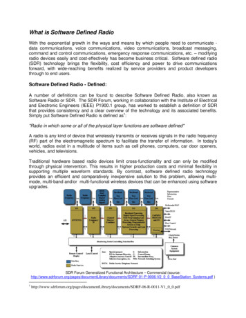
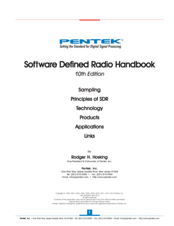
band. Such systems can be quite complex and somewhat out of reach tomost amateurs.One problem has been that unlessyou are a math wizard and proficientin programming C or assembly language, you are out of luck. Each can besomewhat daunting to the amateur aswell as to many professionals. Twoyears ago, I set out to attack this challenge armed with a fascination fortechnology and a 25-year-old, virtually unused electrical engineering degree. I had studied most of the math incollege and even some of the signalprocessing theory, but 25 years is along time. I found that it really was achallenge to learn many of the disciplines required because much of theliterature was written from a mathematician’s perspective.Now that I am beginning to graspmany of the concepts involved in software radios, I want to share with theAmateur Radio community what Ihave learned without using muchmore than simple mathematical concepts. Further, a software radioshould have as little hardware as possible. If you have a PC with a soundcard, you already have most of therequired hardware. With as few asthree integrated circuits you can be upand running with a Tayloe detector—an innovative, yet simple, direct-conversion receiver. With less than adozen chips, you can build a transceiver that will outperform much ofthe commercial gear on the market.Approach the TheoryIn this article series, I have chosen tofocus on practical implementationrather than on detailed theory. Thereare basic facts that must be understoodto build a software radio. However,much like working with integrated circuits, you don’t have to know how tocreate the IC in order to use it in a design. The convention I have chosen is todescribe practical applications followed by references where appropriatefor more detailed study. One of theeasier to comprehend references I havefound is The Scientist and Engineer’sGuide to Digital Signal Processing bySteven W. Smith. It is free for downloadover the Internet at www.DSPGuide.com. I consider it required reading forthose who want to dig deeper intoimplementation as well as theory. I willrefer to it as the “DSP Guide” manytimes in this article series for furtherstudy.So get out your four-function calculator (okay, maybe you need six or14 Jul/Aug 2002seven functions) and let’s get started.But first, let’s set forth the objectivesof the complete SDR design: Keep the math simple Use a sound-card equipped PC to provide all signal-processing functions Program the user interface and allsignal-processing algorithms inVisual Basic for easy developmentand maintenance Utilize the Intel Signal ProcessingLibrary for core DSP routines tominimize the technical knowledgerequirement and development time,and to maximize performance Integrate a direct conversion (D-C)receiver for hardware design simplicity and wide dynamic range Incorporate direct digital synthesis(DDS) to allow flexible frequencycontrol Include transmit capabilities usingsimilar techniques as those used inthe D-C receiver.Analog and Digital Signals inthe Time DomainTo understand DSP we first need tounderstand the relationship betweendigital signals and their analog counterparts. If we look at a 1-V (pk) sinewave on an analog oscilloscope, we seethat the signal makes a perfectlysmooth curve on the scope, no matterhow fast the sweep frequency. In fact,if it were possible to build a scope withan infinitely fast horizontal sweep, itwould still display a perfectly smoothcurve (really a straight line at thatpoint). As such, it is often called a continuous-time signal since it is continuous in time. In other words, there arean infinite number of different voltages along the curve, as can be seen onthe analog oscilloscope trace.On the other hand, if we were tomeasure the same sine wave with adigital voltmeter at a sampling rate offour times the frequency of the sinewave, starting at time equals zero, wewould read: 0 V at 0 , 1 V at 90 , 0 V at180 and –1 V at 270 over one complete cycle. The signal could continueperpetually, and we would still readthose same four voltages over andagain, forever. We have measured thevoltage of the signal at discrete moments in time. The resulting voltagemeasurement sequence is thereforecalled a discrete-time signal.If we save each discrete-time signalvoltage in a computer memory and weknow the frequency at which wesampled the signal, we have a discretetime sampled signal. This is what ananalog-to-digital converter (ADC)does. It uses a sampling clock to measure discrete samples of an incominganalog signal at precise times, and itproduces a digital representation ofthe input sample voltage.In 1933, Harry Nyquist discoveredthat to accurately recover all the components of a periodic waveform, it isnecessary to use a sampling frequencyof at least twice the bandwidth of thesignal being measured. That minimum sampling frequency is called theNyquist criterion. This may be expressed as:f s 2 f bw(Eq 1)where fs is the sampling rate and fbw isthe bandwidth. See? The math isn’t sobad, is it?Now as an example of the Nyquistcriterion, let’s consider human hearing, which typically ranges from 20 Hzto 20 kHz. To recreate this frequencyresponse, a CD player must sample ata frequency of at least 40 kHz. As wewill soon learn, the maximum frequency component must be limited to20 kHz through low-pass filtering toprevent distortion caused by false images of the signal. To ease filter requirements, therefore, CD players usea standard sampling rate of 44,100 Hz.All modern PC sound cards supportthat sampling rate.What happens if the sampled bandwidth is greater than half the samplingrate and is not limited by a low-passfilter? An alias of the signal is producedthat appears in the output along withthe original signal. Aliases can causedistortion, beat notes and unwantedspurious images. Fortunately, aliasfrequencies can be precisely predictedand prevented with proper low-pass orband-pass filters, which are often referred to as anti-aliasing filters, asshown in Fig 1. There are even caseswhere the alias frequency can be usedto advantage; that will be discussedlater in the article.This is the point where most textson DSP go into great detail about whatsampled signals look like above theNyquist frequency. Since the goal ofthis article is practical implementation, I refer you to Chapter 3 of theDSP Guide for a more in-depth discussion of sampling, aliases, A-to-D andFig 1—A/D conversion with antialiasinglow-pass filter.
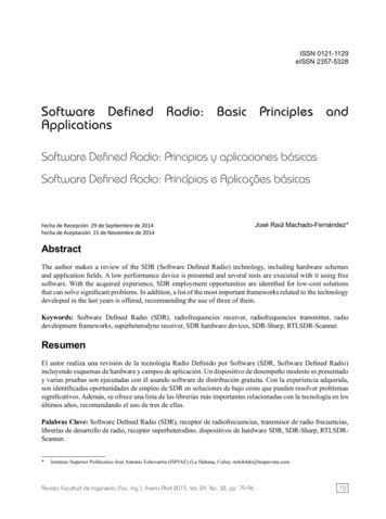
D-to-A conversion. Also refer to Doug Smith’s article, “Signals, Samples, and Stuff: A DSP Tutorial.”1What you need to know for now is that if we adhere to theNyquist criterion in Eq 1, we can accurately sample, process and recreate virtually any desired waveform. Thesampled signal will consist of a series of numbers in computer memory measured at time intervals equal to thesampling rate. Since we now know the amplitude of thesignal at discrete time intervals, we can process the digitized signal in software with a precision and flexibility notpossible with analog circuits.From RF to a PC’s Sound CardOur objective is to convert a modulated radio-frequencysignal from the frequency domain to the time domain forsoftware processing. In the frequency domain, we measureamplitude versus frequency (as with a spectrum analyzer);in the time domain, we measure amplitude versus time (aswith an oscilloscope).In this application, we choose to use a standard 16-bit PCsound card that has a maximum sampling rate of44,100 Hz. According to Eq 1, this means that the maximum-bandwidth signal we can accommodate is 22,050 Hz.With quadrature sampling, discussed later, this can actually be extended to 44 kHz. Most sound cards have built-inantialiasing filters that cut off sharply at around 20 kHz.(For a couple hundred dollars more, PC sound cards arenow available that support 24 bits at a 96-kHz samplingrate with up to 105 dB of dynamic range.)Most commercial and amateur DSP designs use dedicatedDSPs that sample intermediate frequencies (IFs) of 40 kHzor above. They use traditional analog superheterodyne techniques for down-conversion and filtering. With the advent ofvery-high-speed and wide-bandwidth ADCs, it is now possible to directly sample signals up through the entire HFrange and even into the low VHF range. For example, theAnalog Devices AD9430 A/D converter is specified withsample rates up to 210 Msps at 12 bits of resolution and a700-MHz bandwidth. That 700-MHz bandwidth can be usedin under-sampling applications, a topic that is beyond thescope of this article series.The goal of my project is to build a PC-based softwaredefined radio that uses as little external hardware as possible while maximizing dynamic range and flexibility. Todo so, we will need to convert the RF signal to audio frequencies in a way that allows removal of the unwantedmixing products or images caused by the down-conversionprocess. The simplest way to accomplish this while maintaining wide dynamic range is to use D-C techniques totranslate the modulated RF signal directly to baseband.1Notes appear on page 21.Fig 2—A direct-conversion real mixer with a 1.5-kHz low-passfilter.We can mix the signal with an oscillator tuned to the RFcarrier frequency to translate the bandwidth-limited signal to a 0-Hz IF as shown in Fig 2.The example in the figure shows a 14.001-MHz carriersignal mixed with a 14.000-MHz local oscillator to translatethe carrier to 1 kHz. If the low-pass filter had a cutoff of1.5 kHz, any signal between 14.000 MHz and 14.0015 MHzwould be within the passband of the direct-conversion receiver. The problem with this simple approach is that wewould also simultaneously receive all signals between13.9985 MHz and 14.000 MHz as unwanted images withinthe passband, as illustrated in Fig 3. Why is that?Most amateurs are familiar with the concept of sum anddifference frequencies that result from mixing two signals.When a carrier frequency, fc, is mixed with a local oscillator, flo, they combine in the general form:1(Eq 2)[( f c f lo ) ( f c f lo )]2When we use the direct-conversion mixer shown in Fig 2,we will receive these primary output signals:f c f lo f c f lo 14.001 MHz 14.000 MHz 28.001 MHzf c f lo 14.001 MHz 14.000 MHz 0.001 MHzNote that we also receive the image frequency that “foldsover” the primary output signals: f c f lo 14.001 MHz 14.000 MHz 0.001 MHzA low-pass filter easily removes the 28.001-MHz sumfrequency, but the –0.001-MHz difference-frequency imagewill remain in the output. This unwanted image is thelower sideband with respect to the 14.000-MHz carrier frequency. This would not be a problem if there were no signals below 14.000 MHz to interfere. As previously stated,all undesired signals between 13.9985 and 14.000 MHz willtranslate into the passband along with the desired signalsabove 14.000 MHz. The image also results in increasednoise in the output.So how can we remove the image-frequency signals? Itcan be accomplished through quadrature mixing. Phasingor quadrature transmitters and receivers—also calledWeaver-method or image-rejection mixers—have existedsince the early days of single sideband. In fact, my firstSSB transmitter was a used Central Electronics 20A exciter that incorporated a phasing design. Phasing systemslost favor in the early 1960s with the advent of relativelyinexpensive, high-performance filters.To achieve good opposite-sideband or image suppression,phasing systems require a precise balance of amplitude andphase between two samples of the signal that are 90 outFig 3—Output spectrum of a real mixer illustrating the sum,difference and image frequencies.Jul/Aug 2002 15
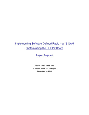
of phase or in quadrature with eachother—“orthogonal” is the term usedin some texts. Until the advent of digital signal processing, it was difficultto realize the level of image rejectionperformance required of modern radiosystems in phasing designs. Sincedigital signal processing allows precise numerical control of phase andamplitude, quadrature modulationand demodulation are the preferredmethods. Such signals in quadratureallow virtually any modulationmethod to be implemented in softwareusing DSP techniques.Give Me I and Q and I CanDemodulate AnythingFirst, consider the direct-conversionmixer shown in Fig 2. When the RF signal is converted to baseband audio using a single channel, we can visualizethe output as varying in amplitudealong a single axis as illustrated inFig 4. We will refer to this as the inphase or I signal. Notice that its magnitude varies from a positive value to anegative value at the frequency of themodulating signal. If we use a diode torectify the signal, we would have created a simple envelope or AM detector.Remember that in AM envelope detection, both modulation sidebandscarry information energy and both aredesired at the output. Only amplitudeinformation is required to fully demodulate the original signal. Theproblem is that most other modulationtechniques require that the phase ofthe signal be known. This is wherequadrature detection comes in. If wedelay a copy of the RF carrier by 90 toform a quadrature (Q) signal, we canthen use it in conjunction with theoriginal in-phase signal and the mathwe learned in middle school to determine the instantaneous phase andamplitude of the original signal.Fig 5 illustrates an RF carrier withthe level of the I signal plotted on thex-axis and that of the Q signal plottedon the y-axis of a plane. This is oftenreferred to in the literature as aphasor diagram in the complex plane.We are now able to extrapolate the twosignals to draw an arrow or phasorthat represents the instantaneousmagnitude and phase of the originalsignal.Okay, here is where you will have touse a couple of those extra functionson the calculator. To compute themagnitude mt or envelope of the signal, we use the geometry of right triangles. In a right triangle, the squareof the hypotenuse is equal to the sum16 Jul/Aug 2002of the squares of the other two sides—according to the Pythagorean theorem. Or restating, the hypotenuse asmt (magnitude with respect to time):mt I t2 Qt2(Eq 3)The instantaneous phase of the signal as measured counterclockwisefrom the positive I axis and may becomputed by the inverse tangent (orarctangent) as follows: Qt (Eq 4) It Therefore, if we measured the instantaneous values of I and Q, wewould know everything we needed toknow about the signal at a given moment in time. This is true whether weare dealing with continuous analogsignals or discrete sampled signals.With I and Q, we can demodulate AMsignals directly using Eq 3 and FMsignals using Eq 4. To demodulateSSB takes one more step. Quadraturesignals can be used analytically to remove the image frequencies and leaveonly the desired sideband.The mathematical equations forquadrature signals are difficult butare very understandable with a littlestudy.2 I highly recommend that youread the online article, “Quadratureφ t tan 1 Fig 4—An in-phase signal (I) on the realplane. The magnitude, m(t), is easilymeasured as the instantaneous peakvoltage, but no phase information isavailable from in-phase detection. This isthe way an AM envelope detector works.Signals: Complex, But Not Complicated,” by Richard Lyons. It can befound at www.dspguru.com/info/tutor/quadsig.htm. The article develops in a very logical manner howquadrature-sampling I/Q demodulation is accomplished. A basic understanding of these concepts is essentialto designing software-defined radios.We can take advantage of the analytic capabilities of quadrature signalsthrough a quadrature mixer. To understand the basic concepts of quadraturemixing, refer to Fig 6, which illustratesa quadrature-sampling I/Q mixer.First, the RF input signal is bandpass filtered and applied to the twoparallel mixer channels. By delayingthe local oscillator wave by 90 , we cangenerate a cosine wave that, in tandem,forms a quadrature oscillator. The RFcarrier, fc(t), is mixed with the respective cosine and sine wave local oscillators and is subsequently low-passfiltered to create the in-phase, I(t), andquadrature, Q(t), signals. The Q(t)Fig 5—I jQ are shown on the complexplane. The vector rotates counterclockπfc. The magnitude andwise at a rate of 2πphase of the rotating vector at any instantin time may be determined through Eqs 3and 4.Fig 6—Quadrature sampling mixer: The RF carrier, fc, is fed to parallel mixers. The localoscillator (Sine) is fed to the lower-channel mixer directly and is delayed by 90 (Cosine)to feed the upper-channel mixer. The low-pass filters provide antialias filtering beforeanalog-to-digital conversion. The upper channel provides the in-phase (I(t)) signal and thelower channel provides the quadrature (Q(t)) signal. In the PC SDR the low-pass filtersand A/D converters are integrated on the PC sound card.
channel is phase-shifted 90 relative tothe I(t) channel through mixing withthe sine local oscillator. The low-passfilter is designed for cutoff below theNyquist frequency to prevent aliasingin the A/D step. The A/D converts continuous-time signals to discrete-timesampled signals. Now that we have theI and Q samples in memory, we canperform the magic of digital signal processing.Before we go further, let me reiterate that one of the problems with thismethod of down-conversion is that itcan be costly to get good opposite-sideband suppression with analog circuits.Any variance in component values willcause phase or amplitude imbalancebetween two channels, resulting in acorresponding decrease in oppositesideband suppression. With analogcircuits, it is difficult to achieve betterthan 40 dB of suppression withoutmuch higher cost. Fortunately, it isstraightforward to correct the analogimbalances in software.Another significant drawback of direct-conversion receivers is that thenoise increases as the demodulated signal approaches 0 Hz. Noise contributions come from a number of sources,such as 1/f noise from the semiconductor devices themselves, 60-Hz and120-Hz line noise or hum, microphonicmechanical noise and local-oscillatorphase noise near the carrier frequency.This can limit sensitivity since mostpeople prefer their CW tones to be below 1 kHz. It turns out that most ofthe low-frequency noise rolls off above1 kHz. Since a sound card can processsignals all the way up to 20 kHz, whynot use some of that bandwidth to moveaway from the low frequency noise? ThePC SDR uses an 11.025-kHz, offsetbaseband IF to reduce the noise to amanageable level. By offsetting thelocal oscillator by 11.025 kHz, we cannow receive signals near the carrierFig 7—FFT output resembles a comb filter:Each bin of the FFT overlaps its adjacentbins just as in a comb filter. The 3-dBpoints overlap to provide linear output. Thephase and magnitude of the signal in eachbin is easily determined mathematicallywith Eqs 3 and 4.frequency without any of the lowfrequency noise issues. This alsosignificantly reduces the effects of local-oscillator phase noise. Once wehave digitally captured the signal, it isa trivial software task to shift the demodulated signal down to a 0-Hz offset.DSP in the Frequency DomainEvery DSP text I have read thus farconcentrates on time-domain filteringand demodulation of SSB signals using finite-impulse-response (FIR) filters. Since these techniques have beenthoroughly discussed in the literature 1, 3, 4 and are not currently used inmy PC SDR, they will not be coveredin this article series.My PC SDR uses the power of thefast Fourier transform (FFT) to do almost all of the heavy lifting in the frequency domain. Most DSP texts use alot of ink to derive the math so that onecan write the FFT code. Since Intel hasso helpfully provided the code in executable form in their signal-processing library,5 we don’t care how to writean FFT: We just need to know how touse it. Simply put, the FFT convertsthe complex I and Q discrete-time signals into the frequency domain. TheFFT output can be thought of as alarge bank of very narrow band-passfilters, called bins, each one measuring the spectral energy within itsrespective bandwidth. The output resembles a comb filter wherein each binslightly overlaps its adjacent binsforming a scalloped curve, as shown inFig 7. When a signal is precisely at thecenter frequency of a bin, there will bea corresponding value only in that bin.As the frequency is offset from thebin’s center, there will be a corresponding increase in the value of theadjacent bin and a decrease in thevalue of the current bin. Mathematical analysis fully describes the relationship between FFT bins,6 but suchis beyond the scope of this article.Further, the FFT allows us to measure both phase and amplitude of thesignal within each bin using Eqs 3 and4 above. The complex version allows usto measure positive and negative frequencies separately. Fig 8 illustratesthe output of a complex, or quadrature, FFT.The bandwidth of each FFT bin maybe computed as shown in Eq 5, whereBWbin is the bandwidth of a single bin,fs is the sampling rate and N is the sizeof the FFT. The center frequency ofeach FFT bin may be determined byEq 6 where fcenter is the bin’s centerfrequency, n is the bin number, fs is thesampling rate and N is the size of theFFT. Bins zero through (N/2)–1 represent upper-sideband frequencies andbins N/2 to N–1 represent lower-sideband frequencies around the carrierfrequency.fs(Eq 5)Nnf(Eq 6)f center sNIf we assume the sampling rate ofthe sound card is 44.1 kHz and thenumber of FFT bins is 4096, then thebandwidth and center frequency ofeach bin would be:BWbin BWbin 44100 10.7666 Hz and4096f center n10.7666 HzWhat this all means is that thereceiver will have 4096, 11-Hz-wideFig 8—Complex FFT output: The output of a complex FFT may be thought of as a seriesof band-pass filters aligned around the carrier frequency, fc, at bin 0. N represents thenumber of FFT bins. The upper sideband is located in bins 1 through (N/2)–1 and thelower sideband is located in bins N/2 to N–1. The center frequency and bandwidth ofeach bin may be calculated using Eqs 5 and 6.Jul/Aug 2002 17
band-pass filters. We can thereforecreate band-pass filters from 11 Hz toapproximately 40 kHz in 11-Hz steps.The PC SDR performs the followingfunctions in the frequency domain after FFT conversion: Brick-wall fixed and variable bandpass filters Frequency conversion SSB/CW demodulation Sideband selection Frequency-domain noise subtraction Frequency-selective squelch Noise blanking Graphic equalization (“tone control”) Phase and amplitude balancing toremove images SSB generation Future digital modes such as PSK31and RTTYOnce the desired frequency-domainprocessing is completed, it is simple toconvert the signal back to the time domain by using an inverse FFT. In thePC SDR, only AGC and adaptive noisefiltering are currently performed in thetime domain. A simplified diagram ofthe PC SDR software architecture isprovided in Fig 9. These conceptswill be discussed in detail in a futurearticle.Sampling RF Signals with theTayloe Detector: A New Twiston an Old ProblemWhile searching the Internet forinformation on quadrature mixing, Iran across a most innovative and elegant design by Dan Tayloe, N7VE.Dan, who works for Motorola, has developed and patented (US Patent#6,230,000) what has been called theTayloe detector. 7 The beauty of theTayloe detector is found in both itsdesign elegance and its exceptionalperformance. It resembles other concepts in design, but appears unique inits high performance with minimalcomponents. 8, 9, 110, 11 In its simplestform, you can build a complete quadrature down converter with only three orfour ICs (less the local oscillator) at acost of less than 10.Fig 10 illustrates a single-balancedversion of the Tayloe detector. It can bevisualized as a four-position rotaryswitch revolving at a rate equal to thecarrier frequency. The 50-Ω antennaimpedance is connected to the rotor andeach of the four switch positions is connected to a sampling capacitor. Sincethe switch rotor is turning at exactlythe RF carrier frequency, each capacitor will track the carrier’s amplitudefor exactly one-quarter of the cycle andwill hold its value for the remainder of18 Jul/Aug 2002Fig 9—SDR receiver software architecture: The I and Q signals are fed from the soundcard input directly to a 4096-bin complex FFT. Band-pass filter coefficients areprecomputed and converted to the frequency domain using another FFT. The frequencydomain filter is then multiplied by the frequency-domain signal to provide brick-wallfiltering. The filtered signal is then converted to the time domain using the inverse FFT.Adaptive noise and notch filtering and digital AGC follow in the time domain.Fig 10—Tayloe detector: The switch rotates at the carrier frequency so that eachcapacitor samples the signal once each revolution. The 0 and 180 capacitorsdifferentially sum to provide the in-phase (I) signal and the 90 and 270 capacitors sumto provide the quadrature (Q) signal.the cycle. The rotating switch willtherefore sample the signal at 0 , 90 ,180 and 270 , respectively.As shown in Fig 11, the 50-Ω impedance of the antenna and the samplingcapacitors form an R-C low-pass filterduring the period when each respective switch is turned on. Therefore,each sample represents the integral oraverage voltage of the signal during itsrespective one-quarter cycle. Whenthe switch is off, each sampling capacitor will hold its value until the nextrevolution. If the RF carrier and therotating frequency were exactly inphase, the output of each capacitorwill be a dc level equal to the averageFig 11—Track and hold sampling circuit:Each of the four sampling capacitors in theTayloe detector form an RC track-and-holdcircuit. When the switch is on, thecapacitor will charge to the average valueof the carrier during its respective onequarter cycle. During the remaining threequarters cycle, it will hold its charge. Thelocal-oscillator frequency is equal to thecarrier frequency so that the output will beat baseband.
value of the sample.If we differentially sum outputs ofthe 0 and 180 sampling capacitorswith an op amp (see Fig 10), the output would be a dc voltage equal to twotimes the value of the individuallysampled values when the switch rotation frequency equals the carrier frequency. Imagine, 6 dB of noise-freegain! The same would be true for the90 and 270 capacitors as well. The0 /180 summation forms the I channel and the 90 /270 summation formsthe Q channel of the quadrature downconversion.As we shift the frequency of the carrier away from the sampling frequency, the values of the invertingphases will no longer be dc levels. Theoutput frequency will vary accordingto the “beat” or difference frequencybetween the carrier and the switch-rotation frequency to provide an accurate representation of all the signalcomponents converted to baseband.Fig 12 provides the schematic for asimple, single-balanced Tayloe detector. It consists of a PI5V331, 1:4 FETdemultiplexer that switches the signalto each of the four sampling capacitors. The 74AC74 dual flip-flop is connected as a divide-by-four Johnsoncounter to provide the two-phase clockto the demultiplexer chip. The outputsof the sampling capacitors are differentially summed through the twoLT1115 ultra-low-noise op amps toform the I and Q outputs, respectively.Note that the impedance of theantenna forms the input resistance forthe op-amp gain as shown in Eq 7. Thisimpedance may vary significantlywith the actual antenna. I use instrumentation amplifiers in my final design to eliminate gain variance withantenna impedance. More informatio
A Software-Defined Radio for the Masses, Part 1 By Gerald Youngblood, AC5OG This series describes a complete PC-based, software-defined radio that uses a sound card and an innovative detector circuit. Mathematics is minimized in the explanation. Come see how it ’s done